Navigating Junctional Diversity in NBS Gene Analysis: Methods, Challenges, and Clinical Translation

Abstract

The analysis of Nucleotide-Binding Site (NBS) genes is fundamental to understanding disease resistance mechanisms in biomedical research. However, the extensive junctional diversity—encompassing sequence variability, domain architecture, and evolutionary divergence—presents significant challenges in accurate gene annotation, functional prediction, and diagnostic application. This article provides a comprehensive framework for researchers and drug development professionals to address these complexities. We explore the foundational principles of NBS gene diversity, detail advanced methodological approaches for robust analysis, present strategies for troubleshooting common pitfalls, and establish validation protocols to ensure biological relevance. By integrating cutting-edge genomic technologies, statistical genetics, and functional assays, this guide aims to enhance the precision of NBS gene studies and accelerate their translation into therapeutic and diagnostic innovations.

Decoding NBS Gene Complexity: Origins and Impact of Junctional Diversity

Junctional diversity refers to the extensive variation created at the junctions of gene segments during recombination and mutational processes in biological systems. This phenomenon is crucial for generating the vast repertoires of antigen receptors in vertebrates and disease resistance genes in plants. In immunological contexts, junctional diversity results from processing of coding ends before ligation, including both base additions and nucleotide loss during V(D)J recombination [1]. This processing accounts for most immunoglobulin and T cell receptor repertoire diversity, allowing recognition of countless pathogens [1].

In plant systems, junctional diversity manifests through domain architecture variations in nucleotide-binding site (NBS) genes, which constitute the largest family of plant resistance (R) genes. These NBS-containing genes exhibit remarkable structural diversity through combinations of various protein domains, creating different binding specificities against pathogens [2] [3]. The NBS domain itself can bind ATP/GTP, facilitating phosphorylation that transmits disease resistance signals downstream in plant immune pathways [3].

Key Concepts and Terminology

Core Definitions

• Junctional Diversity: The molecular variation generated at the junctions of recombining gene segments through nucleotide addition and deletion processes, significantly expanding receptor diversity [1].
• N-Region Diversity: Addition of non-templated nucleotides at coding joints by terminal deoxynucleotidyl transferase (TdT) [1] [4].
• Coding Joint: Formed by joining gene coding segments after recombination signal sequence cleavage [1].
• Signal Joint: Created by joining recombination signal sequences during V(D)J recombination [1].
• NBS-LRR Genes: Nucleotide-binding site leucine-rich repeat genes, the largest family of plant resistance genes providing pathogen recognition capabilities [3] [5].

Molecular Mechanisms Creating Junctional Diversity

Research Reagent Solutions for Junctional Diversity Studies

Table 1: Essential Research Reagents for Junctional Diversity Analysis

Reagent Category	Specific Examples	Experimental Function	Key Considerations
Primer Sets	Degenerate primers for P-loop, Kinase-2, GLPL motifs [6]	Amplification of NBS domains from genomic DNA	Design degeneracy to match sequence diversity; 16 primers can cover most R genes [6]
HMM Profiles	NB-ARC domain (PF00931) [3] [7] [5]	Identification of NBS-containing genes in genomes	Use E-value < 1.0 for initial screening; verify with additional domain analysis [3]
Cloning Systems	Virus-Induced Gene Silencing (VIGS) vectors [2] [5]	Functional validation of NBS-LRR gene function	Enables rapid testing of gene function without stable transformation [5]
Sequence Analysis Tools	MEME Suite, HMMER, OrthoFinder [3]	Identification of conserved motifs and evolutionary relationships	Motif width 6-50 amino acids; bootstrap value 1000 for phylogenetic trees [3]
Structural Analysis	Coiled-coil prediction tools (e.g., Coils) [3]	Identification of CC domains in NBS-LRR proteins	Threshold value of 0.5; CC domains not always identified by Pfam searches [3]

Experimental Protocols for Junctional Diversity Analysis

Genome-Wide Identification of NBS-LRR Genes

Purpose: To systematically identify and classify NBS-containing resistance genes across plant genomes [3] [5].

Methodology:

• Sequence Retrieval: Download genome sequence and annotation files from public databases (NCBI, Phytozome, Plaza) [2].
• HMMER Search: Perform HMMsearch using NB-ARC domain (PF00931) with E-value < 1.0 [3] [5]:

• Domain Verification: Confirm NBS domain presence using Pfam database with E-value threshold of 10^-4 [3].
• Classification: Identify additional domains (TIR, CC, RPW8, LRR) using NCBI CDD and coiled-coil prediction tools [3].
• Manual Curation: Remove redundant genes and verify domain architecture through multiple databases.

Troubleshooting Tip: CC domains may not be detected by standard Pfam searches; use specialized coiled-coil prediction tools with threshold 0.5 [3].

NBS Profiling for Resistance Gene Allele Discovery

Purpose: To capture sequence diversity in NBS domains across multiple cultivars or accessions [6].

Methodology:

• Primer Design: Design degenerate primers complementary to conserved P-loop, Kinase-2, and GLPL motifs within NBS domains [6].
• PCR Amplification: Amplify NBS tags (200-480 bp fragments) from genomic DNA using multiple primer combinations.
• High-Throughput Sequencing: Sequence amplicons using Illumina platforms.
• Read Mapping: Map NBS tags to reference genome, allowing for detection of polymorphisms.
• Variant Analysis: Identify single nucleotide polymorphisms and haplotypes across samples.

Technical Note: 16 carefully designed primers can cover virtually all R genes carrying at least one of the three NBS domain-specific motifs [6].

Functional Validation Using Virus-Induced Gene Silencing

Purpose: To confirm the role of specific NBS-LRR genes in disease resistance [2] [5].

Methodology:

• Candidate Gene Selection: Identify NBS-LRR genes with differential expression in resistant vs. susceptible varieties.
• VIGS Construct Design: Clone 200-300 bp fragment of target gene into TRV-based silencing vector.
• Plant Infiltration: Agro-infiltrate silencing construct into cotyledons or true leaves.
• Pathogen Challenge: Inoculate silenced plants with target pathogen after silencing establishment (typically 2-3 weeks).
• Phenotypic Assessment: Monitor disease symptoms, measure pathogen biomass, and document hypersensitive responses.
• Molecular Confirmation: Verify gene silencing efficiency through qRT-PCR.

Application Example: Silencing of GaNBS (OG2) in resistant cotton demonstrated its role in virus resistance against cotton leaf curl disease [2].

Frequently Asked Questions (FAQs)

Technical Troubleshooting

Q: Why do my degenerate primers fail to amplify expected NBS domains? A: Optimize primer degeneracy based on target species. For potato, 16 primers covering P-loop, Kinase-2 and GLPL motifs successfully amplified nearly all NBS domains [6]. Validate primer functionality through initial PCR on genomic DNA before high-throughput application.

Q: How can I distinguish between functional and non-functional NBS-LRR genes? A: Analyze for intact open reading frames and conserved motif structure. Functional NBS domains typically contain eight conserved motifs with specific order and amino acid conservation [3]. Combine sequence analysis with expression studies - functional genes often show induction upon pathogen challenge [5].

Q: What is the typical number of NBS-LRR genes expected in a plant genome? A: This varies significantly by species. Akebia trifoliata has 73 NBS genes [3], Vernicia fordii has 90 [5], while tobacco has 156 NBS-LRR homologs [7]. The number correlates with genome size and evolutionary history rather than taxonomic classification.

Data Analysis and Interpretation

Q: How do I handle the mapping of NBS tags when working with non-reference genotypes? A: Be aware that mapping inaccuracies can occur due to differences between cultivars and the reference genome, coupled with high NBS domain sequence similarity. This may yield more than the possible 4 alleles per domain in tetraploid species, indicating potential locus intermixing [6]. Use stringent mapping parameters and validate with manual inspection.

Q: What criteria should I use to classify NBS-LRR genes into subfamilies? A: Use a hierarchical approach:

• Identify N-terminal domain (TIR, CC, RPW8, or none)
• Confirm NBS domain integrity
• Detect C-terminal LRR presence
• Classify as TNL, CNL, RNL, TN, CN, or N-type based on combination [7]

Q: How can I identify candidate NBS-LRR genes for specific disease resistance? A: Look for orthologous gene pairs between resistant and susceptible varieties that show distinct expression patterns. For example, Vf11G0978-Vm019719 pair where the resistant ortholog shows upregulated expression during infection while susceptible counterpart does not [5].

Advanced Analysis Techniques

Evolutionary Analysis of NBS Gene Family

Methodology:

• Orthogroup Identification: Use OrthoFinder v2.5.1 with DIAMOND for sequence similarity searches and MCL clustering [2].
• Phylogenetic Construction: Employ maximum likelihood algorithm in FastTreeMP with 1000 bootstrap replicates [2].
• Duplication Analysis: Identify tandem and dispersed duplications as primary forces for NBS expansion [3].

Table 2: NBS-LRR Gene Distribution Across Plant Species

Plant Species	Total NBS Genes	TNL	CNL	RNL	Other	Reference
Akebia trifoliata	73	19	50	4	-	[3]
Vernicia fordii	90	0	12 (CNL)	-	78 (Other NBS)	[5]
Vernicia montana	149	3 (TNL)	9 (CNL)	-	137 (Other NBS)	[5]
Nicotiana benthamiana	156	5	25	4 (RPW8)	122 (Other)	[7]
Common Potato	587-755	Varies	Varies	Varies	Varies	[6]

Expression Analysis and Regulatory Elements

Methodology:

• RNA-seq Data Collection: Retrieve FPKM values from specialized databases (CottonFGD, IPF database) [2].
• Expression Categorization: Group expression data into tissue-specific, abiotic stress, and biotic stress responses.
• Cis-Element Analysis: Identify regulatory elements in promoter regions (1500 bp upstream) using PlantCARE database [7].
• Co-expression Networks: Construct networks to identify regulatory relationships (e.g., VmWRKY64 activating Vm019719) [5].

Nucleotide-binding site (NBS) genes constitute one of the most critical and dynamically evolving gene families in plants, encoding key receptors for pathogen detection and disease resistance. These genes, particularly those belonging to the NBS-LRR (leucine-rich repeat) class, are central to the plant immune system, enabling recognition of diverse pathogens through effector-triggered immunity. The remarkable diversity of NBS genes presents both a scientific opportunity and a technical challenge for researchers. This technical support center addresses the experimental complexities arising from the junctional diversity of NBS genes, focusing specifically on how whole-genome duplication (WGD) and tandem duplication events have driven their expansion and diversification across plant lineages.

The evolutionary mechanisms underlying NBS gene expansion are not merely academic concerns—they directly impact experimental design, data interpretation, and technical troubleshooting in molecular biology research. Studies across multiple plant species have revealed that NBS genes evolve at least 1.5-fold faster at synonymous sites and approximately 2.3-fold faster at nonsynonymous sites compared to flanking non-NBS genes, with gene loss occurring approximately twice as rapidly [8]. This rapid evolutionary dynamic, driven by the combined effects of diversifying selection and frequent sequence exchanges, creates substantial technical challenges for researchers working with these genes [8].

Table 1: Evolutionary Dynamics of NBS Genes Across Plant Species

Evolutionary Parameter	Comparative Rate	Experimental Implications
Synonymous substitution rate	~1.5x higher than non-NBS genes	Complicates primer design and cross-species PCR amplification
Nonsynonymous substitution rate	~2.3x higher than non-NBS genes	Affects protein structure-function analyses and antibody development
Gene loss rate	~2x faster than non-NBS genes	Leads to presence-absence polymorphisms that complicate genotyping
Tandem duplication prevalence	Major expansion mechanism in soybean and Arabidopsis [8] [9]	Creates complex clusters requiring specialized assembly approaches
Segmental duplication contribution	Significant in asparagus and soybean [10] [8]	Necessitates whole-genome context for proper annotation

FAQs: Troubleshooting NBS Gene Analysis

How can I accurately identify and annotate NBS genes in a newly sequenced plant genome?

Challenge: Researchers frequently report incomplete identification of NBS genes, particularly from tandemly duplicated clusters, leading to fragmented assemblies and inaccurate gene models.

Solution: Implement a reiterative BLAST and domain-based identification protocol:

• Initial Homology Search: Use BLASTP with known NBS proteins from closely related species (e.g., Allium sativum for monocots) with cutoff values of 30% identity, 30% query coverage, and E-value < 1×10⁻³⁰ [10].

• Domain Validation: Confirm NBS domains using NCBI's Conserved Domain Database (CDD) with E-value < 0.01 [10].

• Motif Identification: Identify TIR, CC, or LRR motifs using Pfam database, SMART protein motif analysis, and COILS program (threshold 0.9) [10].

• Iterative Searching: Use newly identified sequences as subsequent queries until no additional members are detected [10].

Troubleshooting Tip: If encountering high false-negative rates in complex genomes, supplement with HMMER searches using PfamScan and the Pfam-A.hmm model with default e-value (1.1e-50) [2]. This approach identified 12,820 NBS-domain-containing genes across 34 species in a recent study, capturing both classical and species-specific structural patterns [2].

What strategies effectively resolve complex NBS gene clusters arising from tandem duplications?

Challenge: Tandemly duplicated NBS genes exhibit high sequence similarity, causing assembly fragmentation and misassembly that obscures true gene copy number and organization.

Solution: Employ a multi-platform sequencing approach:

• Long-Read Sequencing: Utilize PacBio or Nanopore sequencing to span repetitive regions and resolve complex clusters where ~50% of NBS genes reside in clusters [10].

• Cluster Definition Parameters: Define clusters using established criteria: minimum 2 genes, intergene distance <200 kb, and no more than 8 non-NBS genes between neighboring NBS-LRR genes [10].

• Gene Family Classification: Apply the coverage/identity threshold method: aligned region >70% of longer gene with >70% identity [10].

• Expression Validation: Use transcriptome sequencing to confirm transcribed genes and correct annotation boundaries.

Troubleshooting Tip: For persistent gaps in cluster regions, employ chromosome conformation capture (Hi-C) to scaffold clusters and validate physical organization. In asparagus, chromosome 6 was found to be significantly NBS-enriched, with one cluster hosting 10% of all NBS genes [10].

How do I distinguish between functional NBS genes and pseudogenes?

Challenge: NBS gene families contain numerous pseudogenes that complicate functional analyses and lead to false positives in resistance gene discovery.

Solution: Implement a multi-tiered filtering strategy:

• Transcriptional Evidence: Analyze RNA-seq data from multiple tissues and stress conditions to confirm expression [2] [10].

• Open Reading Frame Analysis: Verify complete ORFs without premature stop codons or frameshift mutations.

• Domain Integrity: Confirm presence and order of essential domains (NBS, LRR, TIR/CC) using Pfam and SMART.

• Evolutionary Conservation: Assess selection pressures—functional genes typically show signatures of positive selection rather than neutral evolution.

Troubleshooting Tip: Be aware that some pseudogenes may be transcribed and even regulated by miRNAs. In Gossypium hirsutum, genetic variation analysis identified 6,583 unique variants in tolerant accessions versus 5,173 in susceptible ones, highlighting the importance of functional validation [2].

What methods reliably detect recent versus ancient duplication events in NBS genes?

Challenge: Determining the timing and mechanism of duplication events is essential for understanding NBS gene evolution but requires specialized analytical approaches.

Solution: Apply phylogenetic and synteny-based methods:

• Sequence Similarity Thresholds: Estimate temporal differences using proportion of multigene families across 80-90% similarity/coverage thresholds [10].

• Synonymous Substitution Rates: Calculate Ks values for paralogous pairs—lower Ks values indicate more recent duplications.

• Synteny Analysis: Identify segmental duplications by comparing genomic regions flanking NBS genes (15 genes on each side) and detecting >5 syntenic gene pairs with E-value < 1×10⁻¹⁰ [10].

• Phylogenetic Reconstruction: Construct gene trees using maximum likelihood methods based on NBS domain sequences (from P-loop to MHDV) [10].

Troubleshooting Tip: For recent tandem duplications, expect to find significant sequence exchanges coupled with positive selection, as observed in most tandem-duplicated NBS gene families in soybean [8].

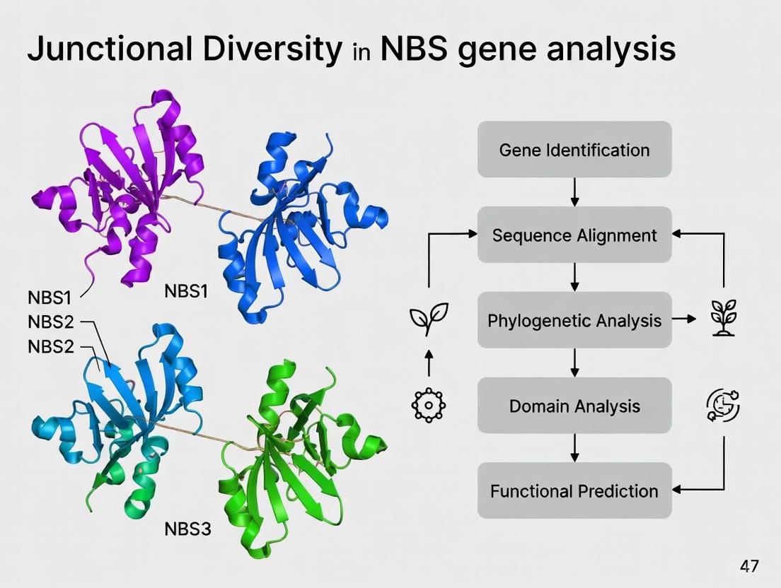
Diagram 1: Experimental workflow for comprehensive NBS gene analysis, highlighting key stages where specific troubleshooting approaches are essential.

Experimental Protocols for NBS Gene Characterization

Orthogroup Analysis and Evolutionary Diversification

Purpose: To classify NBS genes into evolutionarily meaningful groups and trace their diversification across species.

Methodology:

• Sequence Collection: Compile NBS protein sequences from species of interest.
• Orthogroup Delineation: Use OrthoFinder v2.5.1 with DIAMOND for sequence similarity searches and MCL clustering algorithm [2].
• Phylogenetic Reconstruction: Perform multiple sequence alignment with MAFFT 7.0 and construct gene trees using maximum likelihood algorithm in FastTreeMP with 1000 bootstrap replicates [2].
• Orthogroup Classification: Identify core (conserved across species) and unique (species-specific) orthogroups.

Technical Notes: This approach identified 603 orthogroups with both core (OG0, OG1, OG2) and unique (OG80, OG82) orthogroups showing tandem duplications in a recent pan-species analysis [2]. Expression profiling revealed putative upregulation of OG2, OG6, and OG15 under various biotic and abiotic stresses [2].

Expression Profiling Under Stress Conditions

Purpose: To link specific NBS genes to stress responses and identify candidates for functional validation.

Methodology:

• Data Collection: Retrieve RNA-seq data from public databases (IPF, CottonFGD, CottonGen) or generate new data [2].
• Data Categorization: Organize expression data into three types: (1) tissue-specific, (2) abiotic stress-specific, and (3) biotic stress-specific.
• FPKM Extraction: Obtain FPKM values using gene accessions as query IDs.
• Differential Analysis: Compare expression between susceptible and tolerant genotypes under stress conditions.

Technical Notes: In cotton, this approach identified differential NBS expression between Coker 312 (susceptible) and Mac7 (tolerant) accessions in response to cotton leaf curl disease [2].

Functional Validation via Virus-Induced Gene Silencing

Purpose: To confirm the functional role of candidate NBS genes in disease resistance.

Methodology:

• Candidate Selection: Choose NBS genes with stress-responsive expression patterns.
• VIGS Construct Design: Design TRV-based silencing constructs targeting candidate genes.
• Plant Inoculation: Infiltrate plants with Agrobacterium containing VIGS constructs.
• Phenotypic Assessment: Challenge silenced plants with pathogens and quantify disease symptoms.
• Molecular Verification: Confirm gene silencing and measure pathogen titers.

Technical Notes: Silencing of GaNBS (OG2) in resistant cotton demonstrated its putative role in virus tittering, validating its function in disease resistance [2].

Table 2: NBS Gene Duplication Patterns Across Plant Species

Plant Species	Total NBS Genes	Tandem Duplication	Segmental Duplication	Key References
Arabidopsis thaliana	Not specified	Major driver for gene family expansion [9]	Contributes to gene family evolution [9]	[9]
Soybean (Glycine max)	Not specified	More abundant than segmental duplicates [8]	Revealed by syntenic homoeologs [8]	[8]
Garden asparagus	68 proteins (49 loci)	Present (specific clusters)	Present (across multiple chromosomes)	[10]
Multiple species (34 plants)	12,820 genes	Tandem duplications in orthogroups	Inferred from phylogenetic patterns	[2]

Research Reagent Solutions for NBS Gene Studies

Table 3: Essential Research Reagents and Resources for NBS Gene Analysis

Reagent/Resource	Specific Application	Function in NBS Research	Example Sources
OrthoFinder	Evolutionary analysis	Discerns orthogroups and evolutionary relationships	[2]
MEME Suite	Motif discovery	Identifies conserved protein motifs in NBS genes	[10]
Pfam/ SMART databases	Domain architecture analysis	Classifies NBS genes based on domain composition	[2] [10]
NCBI CDD	Domain verification	Validates NBS domain presence with statistical support	[10]
MEGA software	Phylogenetic reconstruction	Builds evolutionary trees of NBS gene families	[10]
VIGS vectors	Functional validation	Tests disease resistance function of candidate NBS genes	[2]

Diagram 2: Characteristics and outcomes of tandem versus segmental duplication mechanisms in NBS gene evolution, highlighting their distinct experimental implications.

Advanced Technical Considerations

miRNA Regulation of NBS Genes

The expansion and evolution of NBS genes is intricately linked to their regulation by miRNAs. At least eight families of miRNAs are known to target NBS-LRRs, typically binding to conserved regions like the P-loop motif [11]. This regulatory relationship represents an important co-evolutionary system that balances the benefits and costs of maintaining large NBS-LRR repertoires [11]. When designing functional studies, researchers should consider that:

• miRNAs typically target highly duplicated NBS-LRRs, while heterogeneous NBS-LRRs are rarely targeted [11].
• Duplicated NBS-LRRs periodically give birth to new miRNAs, with most targeting the same conserved protein motifs [11].
• Nucleotide diversity in the wobble position of codons in the target site drives miRNA diversification [11].

Evolutionary Rate Variation Among NBS Subclasses

Not all NBS genes evolve at the same rate, creating additional experimental considerations. TIR-NBS-LRR genes (TNLs) exhibit higher nucleotide substitution rates than non-TNLs, indicating distinct evolutionary patterns [8]. This differential evolution affects primer design, phylogenetic analysis, and functional inference. Researchers should:

• Subclassify NBS genes before evolutionary analysis
• Use subclass-specific evolutionary rate models
• Consider distinct conservation patterns when designing cross-species experiments

The junctional diversity of NBS genes, driven by the complementary forces of whole-genome and tandem duplication events, represents both a challenge and opportunity for plant disease resistance research. The troubleshooting guides and experimental protocols provided here address the most common technical hurdles researchers face when working with these dynamically evolving gene families. By implementing these standardized approaches—from accurate gene identification and cluster resolution to functional validation and evolutionary analysis—researchers can more effectively navigate the complexity of NBS gene families and advance our understanding of plant immunity mechanisms.

The continued refinement of these methodologies, particularly through the integration of long-read sequencing, multi-omics approaches, and advanced bioinformatics, will further enhance our ability to decipher the evolutionary drivers of NBS expansion and harness these genes for crop improvement. As evidenced by recent studies in asparagus, soybean, cotton, and multiple other species, the strategic application of these technical solutions enables meaningful progress despite the inherent challenges of working with these rapidly evolving, duplication-rich genes.

Nucleotide-binding site (NBS) genes constitute the largest and most crucial family of plant disease resistance (R) genes, playing a vital role in pathogen recognition and defense activation. Your research on their structural classification must account for significant junctional diversity—variations in domain architecture, gene structure, and sequence motifs that arise from evolutionary processes like tandem duplications, domain shuffling, and selective pressures. This diversity presents both challenges in consistent classification and opportunities for understanding plant-pathogen co-evolution.

The following sections provide a comprehensive technical framework to support your experiments, from basic classification to advanced functional characterization, with special attention to troubleshooting common issues encountered when handling this gene family's inherent diversity.

Core Concepts: Classical and Species-Specific NBS Architectures

What are the primary structural classes of NBS genes?

NBS genes are primarily classified based on their protein domain architecture. The classical classification system has been established through comparative genomic studies across multiple plant species [12] [13] [14].

Table 1: Classical Structural Classification of NBS Genes

Category	Subfamily	Domain Architecture	Key Features	Functional Role
Typical NBS-LRR	TNL	TIR-NBS-LRR	Contains TIR domain at N-terminus	Pathogen recognition, signal transduction
	CNL	CC-NBS-LRR	Contains coiled-coil domain at N-terminus	Pathogen recognition, signal transduction
	RNL	RPW8-NBS-LRR	Contains RPW8 domain at N-terminus	Defense signal transduction
Irregular NBS	TN	TIR-NBS	Lacks LRR domain	Regulatory or adapter functions
	CN	CC-NBS	Lacks LRR domain	Regulatory or adapter functions
	N	NBS	Contains only NBS domain	Regulatory or adapter functions

What species-specific architectural variations should I expect?

Beyond classical architectures, your research will encounter species-specific structural patterns that reflect lineage-specific adaptations. Recent pan-genomic studies reveal that NBS genes exhibit significant presence-absence variation (PAV), distinguishing conserved "core" subgroups from highly variable "adaptive" subgroups [15].

In pepper (Capsicum annuum), researchers identified 252 NBS-LRR genes with unusual distribution: 248 nTNLs (non-TIR NBS-LRR) and only 4 TNLs, with 200 genes lacking both CC and TIR domains [13]. This represents a dramatic shift from the typical distribution observed in model plants like Arabidopsis.

In Akebia trifoliata, the NBS gene family is remarkably small with only 73 members, containing 50 CNL, 19 TNL, and 4 RNL genes [16]. This compact repertoire suggests species-specific evolutionary constraints.

Orchids demonstrate another pattern, with complete absence of TNL-type genes across multiple species (Dendrobium officinale, D. nobile, D. chrysotoxum, P. equestris, V. planifolia, and A. shenzhenica) [17], indicating TIR domain degeneration is common in monocots.

Troubleshooting Common Experimental Challenges

How can I resolve inconsistent domain annotation in my NBS gene predictions?

Problem: Different bioinformatics tools (Pfam, SMART, CDD) yield conflicting domain annotations for the same NBS gene sequences.

Solution: Implement a consensus approach with multiple verification steps:

• Primary identification: Use HMMER with NB-ARC domain (PF00931) at E-value < 1×10⁻²⁰ [14] [7]
• Domain verification: Cross-validate with Pfam, SMART, and conserved domain database (CDD)
• Coiled-coil prediction: Use Coiledcoil with threshold 0.5 (CC domains often missed by Pfam) [16]
• Manual curation: Verify boundary positions and domain integrity

Preventive measures: Establish consistent parameter settings across all analyses and use curated reference sequences from closely related species for comparison.

Why do my phylogenetic trees show unstable topologies with NBS sequences?

Problem: Inconsistent tree topologies and low bootstrap values when reconstructing NBS gene evolutionary relationships.

Root causes and solutions:

• Rapid evolution: NBS genes, especially LRR domains, evolve rapidly. Use only the conserved NBS domain for phylogenetic analysis [13]
• Recombination hotspots: NBS genes are prone to recombination. Implement recombination detection (e.g., RDP4) and analyze recombinant regions separately
• Incomplete sequences: Use only full-length domains (TIR-NBS-LRR, CC-NBS-LRR, etc.) for reliable phylogeny [7]
• Appropriate models: Use Whelan and Goldman model with frequency correction for NBS domains [14]

How should I handle non-canonical NBS architectures in my annotation pipeline?

Problem: Your pipeline misses or misclassifies genes with unusual domain combinations like TIR-NBS-TIR-Cupin_1 or NLNLN architectures.

Solution: Expand your classification system to accommodate both classical and species-specific patterns:

• Custom HMM profiles: Develop lineage-specific HMMs based on manually curated examples
• Motif-based classification: Use MEME with 6-50 amino acid width to identify conserved motifs beyond core domains [16] [14]
• Structural validation: Correlate gene structures with exon-intron patterns—CNLs typically have fewer exons than TNLs [16]

Experimental Protocols for Comprehensive NBS Gene Analysis

Protocol 1: Genome-Wide Identification and Classification of NBS Genes

Materials and Reagents:

• Genomic sequence and annotation files (GFF3)
• HMMER software (v3.3.2)
• Pfam database (current version)
• MEME Suite (v5.4.1)
• TBtools or custom scripting environment

Step-by-Step Methodology:

• Initial identification: Perform HMMsearch against target genome using NB-ARC domain (PF00931) with E-value < 1×10⁻²⁰ [14]
• Domain verification: Submit candidate sequences to Pfam, SMART, and CDD for domain validation
• Classification: Categorize genes based on presence/absence of TIR, CC, RPW8, and LRR domains
• Motif discovery: Identify conserved motifs using MEME with parameters: motif count=10, width=6-50 amino acids [16]
• Gene structure analysis: Extract exon-intron information from GFF3 files and visualize with TBtools

Protocol 2: Evolutionary and Expression Analysis of NBS Genes

Materials and Reagents:

• Multiple genome sequences for comparative analysis
• RNA-seq data under stress conditions
• MEGA software (v7.0+)
• Expression analysis tools (DESeq2, edgeR)

Methodology:

• Phylogenetic reconstruction: Align protein sequences using ClustalW, construct tree with Maximum Likelihood method (Whelan and Goldman model, 1000 bootstrap replicates) [14]
• Selection pressure analysis: Calculate Ka/Ks ratios using codeml in PAML package
• Expression profiling: Analyze RNA-seq data to identify NBS genes responsive to pathogens or hormone treatments
• cis-element analysis: Extract 1.5kb promoter regions and identify regulatory elements using PlantCARE database [14]

Visualization of NBS Gene Classification Workflow

The following diagram illustrates the comprehensive workflow for structural classification of NBS genes, integrating both classical and species-specific architectures:

Research Reagent Solutions for NBS Gene Analysis

Table 2: Essential Research Reagents and Computational Tools for NBS Gene Studies

Category	Item/Software	Specific Function	Application Notes
Bioinformatics Tools	HMMER v3.3	Hidden Markov Model searches	Core tool for initial NBS gene identification [14]
	MEME Suite v5.4.1	Motif discovery and analysis	Identifies conserved motifs beyond core domains [16]
	MEGA v7.0+	Phylogenetic analysis	Maximum Likelihood trees with bootstrap testing [14]
	TBtools	Genomic data visualization	Integrates multiple analysis functions [16]
Databases	Pfam Database	Protein domain families	NB-ARC domain (PF00931) as primary reference [14]
	PlantCARE	cis-element prediction	Identifies regulatory elements in promoter regions [14]
	CDD (NCBI)	Conserved domain identification	Validates domain predictions from multiple sources [16]
Experimental Materials	RNA-seq libraries	Expression profiling	Essential for stress-responsive NBS gene identification [17]
	VIGS vectors	Functional validation	Virus-induced gene silencing for gene function studies [12]

Advanced Technical Considerations

How does junctional diversity impact functional studies of NBS genes?

Junctional diversity in NBS genes—created by domain shuffling, exon/intron structure variation, and presence-absence polymorphisms—directly affects your functional characterization outcomes. When designing functional studies:

• Consider architectural context: A CNL gene in a cluster may have different functions than a singleton CNL with identical domains [13]
• Account for expression variation: Structural variants (SVs) significantly impact gene expression patterns independent of domain composition [15]
• Validate subcellular localization: Predict localization using CELLO v.2.5 and Plant-mPLoc, as NBS proteins localize to cytoplasm (77.6%), plasma membrane (21.2%), or nucleus (7.7%) [14]

What analytical strategies best handle the "core-adaptive" model of NBS gene evolution?

Recent pan-genomic analyses support a "core-adaptive" model where some NBS subgroups are conserved across accessions while others show extensive presence-absence variation [15]. To address this:

• Implement pan-genome analysis: Analyze multiple genomes/accessions of your target species to distinguish core and adaptive NBS genes
• Correlate duplication mechanisms with selection pressures: Whole-genome duplication derived genes typically show strong purifying selection (low Ka/Ks), while tandem/segmental duplicates often show relaxed or positive selection [15]
• Map gene clusters: 54% of pepper NBS-LRR genes are physically clustered (47 clusters across chromosomes) [13]—these clusters are hotspots for functional innovation

By integrating these specialized approaches with the fundamental protocols above, your research on NBS gene structural classification will effectively address both classical architectures and the dynamic, species-specific variations that define this crucial gene family.

The Functional Spectrum of NBS Domains in Disease Resistance Pathways

NBS-LRR Gene Identification & Classification Troubleshooting

FAQ: What are the common types of NBS-LRR genes I might identify, and how are they classified? NBS-LRR genes are primarily classified based on their variable N-terminal domains. The two major subfamilies are TIR-NBS-LRR (TNL) and CC-NBS-LRR (CNL), defined by the presence of Toll/interleukin-1 receptor (TIR) or coiled-coil (CC) motifs, respectively [18]. A third, smaller subclass is the RPW8-NBS-LRR (RNL) [19]. Additionally, "irregular" types exist that lack the LRR domain entirely, such as TN (TIR-NBS), CN (CC-NBS), and N (NBS-only) proteins, which may function as adaptors or regulators for the typical types [7].

Troubleshooting Guide: My HMM search is returning too many false positives. How can I improve accuracy?

• Problem: Initial HMMER search results include non-NBS-LRR proteins.
• Solution: A multi-step validation protocol is required.
  • Initial Search: Use HMMER with the NB-ARC domain (PF00931) as a query, setting a strict expectation value (e.g., E-value < 1*10⁻²⁰) [7].
  • Remove Redundancy: Manually remove duplicate genes from the candidate list.
  • Domain Validation: Submit the remaining candidate sequences to Pfam and the NCBI Conserved Domain Database (CDD) to confirm the presence of both the NBS domain and the N-terminal domain (CC, TIR, or RPW8). Use an E-value cutoff of 10⁻⁴ for confirmation [19].
  • Structure Verification: Use tools like SMART to analyze domain architecture and ensure the complete presence of the NBS domain [7].

FAQ: Why does the number of NBS-LRR genes vary so dramatically between species? The NBS-LRR family evolves rapidly through frequent gene duplication and loss events [19]. For example, a study in Rosaceae species revealed distinct evolutionary patterns, such as "continuous expansion" in rose and "expansion followed by contraction" in strawberry, leading to significant differences in gene number even among closely related species [19]. In tung trees, Vernicia montana has 149 NBS-LRR genes, while its susceptible counterpart, Vernicia fordii, has only 90, partly due to the loss of specific LRR domains in V. fordii [5].

Experimental Protocols for Functional Analysis

Protocol 1: Virus-Induced Gene Silencing (VIGS) for Functional Validation This protocol is used to knock down a candidate NBS-LRR gene to test its role in disease resistance [5].

• Candidate Gene Selection: Identify target NBS-LRR genes through transcriptome data or orthologous analysis. For example, the orthologous pair Vf11G0978/Vm019719 was selected due to its differential expression during Fusarium wilt infection [5].
• Vector Construction: Clone a 200-300 bp specific fragment of the target gene into a VIGS vector (e.g., TRV-based vector).
• Plant Infiltration: Transform the construct into Agrobacterium tumefaciens and infiltrate the bacteria into the leaves of young plants (e.g., 2-week-old seedlings of Nicotiana benthamiana or your species of interest).
• Pathogen Challenge: After granting 2-3 weeks for gene silencing to establish, challenge the plants with the target pathogen.
• Phenotypic Assessment: Monitor and record disease symptoms over time. Compare the disease progression in silenced plants against control plants (e.g., transformed with an empty vector).
• Molecular Verification: Use qRT-PCR to confirm the reduction of target gene expression in silenced plants, linking the observed phenotype to the specific gene knockdown [5].

Protocol 2: Analyzing Intramolecular Interactions in NBS-LRR Proteins This protocol, based on the study of the potato Rx protein, tests functional complementation between separate protein domains [20].

• Construct Design: Create expression clones for separate domains of the NBS-LRR protein (e.g., CC-NBS, LRR, CC, NBS-LRR). Ensure these are epitope-tagged (e.g., HA-tag) for detection.
• Transient Co-expression: Express different combinations of these domain constructs in a model system like Nicotiana benthamiana leaves via Agrobacterium-mediated transformation.
• Elicitor Trigger: Co-express the constructs with the known pathogen elicitor (e.g., Potato Virus X Coat Protein for Rx).
• Hypersensitive Response (HR) Assay: Observe for a rapid, localized cell death response (HR), which indicates successful complementation and functional reconstitution of the resistance protein.
• Co-immunoprecipitation (Co-IP): Physically validate the interaction between domains. Immunoprecipitate one tagged domain and probe for the presence of the other interacting domain via western blot.
• Key Control: Test the requirement of a functional P-loop motif in the NBS domain, as the interaction between CC and NBS-LRR is P-loop dependent, whereas the interaction between CC-NBS and LRR is not [20].

Data Presentation: Quantitative Summaries

Table 1: NBS-LRR Gene Family Size and Composition Across Plant Species

Species	Total NBS-LRR Genes	TNL	CNL	RNL	NL	TN	CN	N	Reference
Nicotiana benthamiana (Tobacco)	156	5	25	Not Specified	23	2	41	60	[7]
Vernicia montana (Tung Tree)	149	3	9	Not Specified	12	7	87	29	[5]
Vernicia fordii (Tung Tree)	90	0	12	Not Specified	12	0	37	29	[5]
Arabidopsis thaliana	~150	~62	~69	~7	-	~21	~5	-	[18]

Table 2: Key Research Reagent Solutions for NBS-LRR Studies

Research Reagent / Tool	Function / Application in NBS-LRR Research
HMMER/Pfam (PF00931)	Identifies candidate NBS-LRR homologs in a genome via hidden Markov model searches for the NB-ARC domain [7] [19].
TRV-based VIGS Vector	A virus-induced gene silencing system used to knock down the expression of candidate NBS-LRR genes to test their function in disease resistance [5].
Co-immunoprecipitation (Co-IP)	Validates physical interactions between different domains of an NBS-LRR protein or with downstream signaling partners [20].
MEME Suite	Discovers conserved protein motifs within the NBS and other domains of NBS-LRR proteins, aiding in phylogenetic and functional analysis [7].
Agrobacterium tumefaciens (Strain GV3101)	Used for transient gene expression in plants, essential for protocols like VIGS, HR assays, and subcellular localization [20].

Signaling Pathway & Experimental Workflow Visualization

Diagram 1: NBS-LRR protein acts as a molecular switch. Effector perturbation of a guarded host protein triggers a conformational change in the NBS domain from ADP-bound (inactive) to ATP-bound (active), initiating immune signaling [20] [18].

Diagram 2: A standard experimental workflow for the genome-wide identification and functional characterization of NBS-LRR genes, from bioinformatics to experimental validation [7] [5].

Addressing Junctional Diversity in Analysis

FAQ: How does "junctional diversity" — the variation in domain composition — impact my functional analysis? Junctional diversity, resulting from the presence or absence of domains like TIR, CC, or LRR, creates functionally distinct NBS-LRR proteins. This diversity is not noise but a functional feature [7] [5].

• Typical NBS-LRRs (TNL, CNL): Usually serve as primary sensors that trigger resistance pathways by recognizing pathogen effectors [7] [19].
• Irregular Types (TN, CN, N): Often lack the LRR domain and may function as adaptors or regulators, working in concert with typical NBS-LRRs to modulate immune signaling [7].
• RNL Proteins: Typically do not function as primary R genes but act downstream to transduce defense signals from TNLs and CNLs [19].

Troubleshooting Guide: My candidate NBS-LRR gene lacks an LRR domain. Is it still a valid R gene candidate?

• Problem: An identified NBS-containing gene is classified as an "N," "CN," or "TN" type, lacking the canonical LRR domain responsible for specific recognition.
• Solution: Yes, it is still a valid candidate, but its hypothesized function shifts. Instead of direct pathogen recognition, it may be a key signaling component.
  • Experimental Adjustment: Design interaction studies (e.g., Yeast-Two-Hybrid, Co-IP) to test if your candidate protein physically associates with full-length NBS-LRR proteins.
  • Genetic Analysis: Use VIGS to knock down your candidate and test whether it disrupts the function of known R genes in your pathosystem. An irregular-type NBS-LRR may be essential for the resistance mediated by a typical NBS-LRR partner.

For researchers and drug development professionals working in genomics, population-specific genetic databases are indispensable tools. These repositories are crucial for understanding the genetic basis of diseases, developing targeted therapies, and advancing precision medicine. However, significant gaps and limitations in the current landscape of these databases directly impact the reliability and applicability of research findings, particularly in specialized areas like the analysis of junctional diversity in Next-Generation Sequencing (NGS) data.

Junctional diversity refers to the DNA sequence variations introduced by the improper joining of gene segments during processes like V(D)J recombination, which is fundamental for generating diversity in the vertebrate immune system [21]. Accurate analysis of this diversity depends on high-quality, population-specific reference data. This technical support center provides targeted troubleshooting guidance to help scientists identify and work around database limitations in their genetic analysis workflows.

Quantitative Analysis of Database Gaps

A systematic evaluation of 42 National and Ethnic Mutation Frequency Databases (NEMDBs) reveals critical shortcomings that researchers must account for in their experimental design. The table below summarizes the core quantitative findings from a 2025 systematic review [22].

Table 1: Key Quantitative Gaps Identified in National and Ethnic Mutation Frequency Databases (NEMDBs)

Deficiency Category	Percentage of Databases Affected	Raw Number (out of 42)	Primary Impact on Research
Non-standardized Data Formats	70%	29/42	Hinders automated data integration, cross-database queries, and comparative analysis.
Incomplete or Outdated Data	50%	21/42	Risks basing conclusions on incomplete variant spectra or obsolete information.
Gaps in Cross-Ethnic Comparison Data	60%	25/42	Limits understanding of allele frequency differences across populations, reducing translational relevance.

FAQs: Addressing Common Researcher Challenges

Q1: My analysis of immune receptor junctional diversity shows inconsistent results across different populations. Could underlying database gaps be a factor?

Yes, this is a common issue. Junctional diversity is highly dependent on the genetic background of the population from which the sample is drawn [23]. If the reference database used for annotation or frequency filtering lacks comprehensive data from your population of interest, it can lead to several problems:

• Misclassification of Common Variants: A variant that is common in one population but absent or rare in another may be incorrectly flagged as a novel or significant finding if the database is biased toward the latter population.
• Inaccurate Frequency Filtering: Pipeline filters that remove common polymorphisms rely on accurate population frequency data. Gaps can cause genuine, population-specific signals to be filtered out or, conversely, allow technical artifacts to persist.

Q2: What are the specific implications of these database gaps for researching disorders related to V(D)J recombination?

V(D)J recombination is a primary mechanism for generating antibody and T-cell receptor diversity [21]. Research into its disorders relies on establishing normal baseline junctional diversity, which is population-dependent. Database gaps can directly impact:

• Disease Association Studies: The ability to correlate specific junctional sequences with disease susceptibility or resistance is compromised if the natural variation within the studied cohort is not properly represented in reference data.
• Diagnostic Assay Development: Assays designed to detect aberrant recombination events may have reduced sensitivity or specificity if they are calibrated against a non-representative genetic background [24].

Q3: What practical steps can I take to mitigate the risk of outdated data in my workflow?

Proactive verification is key. Before beginning an analysis, researchers should:

• Check Database Timestamps: Note the last update date for any public database used.
• Consult Multiple Sources: Cross-reference findings against multiple databases (e.g., ClinVar, dbSNP, and population-specific NEMDBs) to triangulate data reliability [22].
• Prioritize Active Databases: Give preference to databases developed on open-source platforms like LOVD, which have been shown to have a 40% increase in usability and are often more regularly maintained [22].

Troubleshooting Guides for Database-Related Experimental Issues

Problem: Inconsistent Variant Calls in Population Cohorts

Potential Cause and Solution:

• Cause: The reference database or allele frequency filter is biased and does not represent the genetic diversity of your cohort.
• Solution: Implement a tiered analysis approach.
  • Initial Calling: Perform variant calling using standard public databases.
  • Cohort-Specific Filtering: Establish a "internal frequency" within your own cohort dataset. A variant that appears at a high frequency within your cohort but is absent from reference databases may still be a real, population-specific variant.
  • Validation: Confirm these population-specific variants using an orthogonal method, such as Sanger sequencing.

Problem: Failed Validation of Apparent Novel Variants from NGS Data

Potential Cause and Solution:

• Cause: The "novel" variant is, in fact, a common polymorphism in a specific population that is missing from the database used for annotation.
• Solution:
  • Check Broader Databases: Query the variant in larger, more diverse aggregate databases like gnomAD to see if it has been reported in any population.
  • Literature Search: Conduct a thorough search of scientific literature for studies focusing on the gene or region in your population of interest.
  • Collaborate: Reach out to research consortia or institutions that specialize in the genetic study of the relevant population.

Experimental Protocol: Validating Population-Specific Junctional Diversity

This protocol outlines a method to confirm and characterize suspected population-specific junctional diversity variants identified through NGS, accounting for potential database gaps.

Method: Sanger Sequencing Validation and Cloning

Background: Junctional diversity in immunoglobin and T-cell receptor genes arises from the imprecise joining of V (variable), D (diversity), and J (joining) gene segments, coupled with the random addition (P and N nucleotides) and subtraction of nucleotides [21] [25]. This process can generate sequences not found in germline databases.

Materials (Research Reagent Solutions):

• Primers: Specifically designed to flank the V-D-J region of interest.
• PCR Reagents: High-fidelity DNA polymerase (e.g., Q5 from NEB #M0491) to minimize PCR-induced errors [26].
• Cloning Vector: T/A-cloning ready vector (e.g., pCR2.1 from Invitrogen).
• Competent E. coli: recA- strain such as NEB 5-alpha (NEB #C2987) to prevent plasmid recombination [27].
• Sanger Sequencing Reagents.

Procedure:

• PCR Amplification: Amplify the target junctional region from genomic or cDNA using high-fidelity polymerase. Optimize conditions to avoid smear patterns or non-specific bands [28].
• Gel Purification: Excise and purify the correct PCR amplicon from an agarose gel.
• Cloning: Ligate the purified PCR product into a T/A-cloning vector and transform into competent E. coli. This step is critical to separate individual molecular sequences for analysis.
• Colony Screening: Pick multiple bacterial colonies (minimum of 20-50) and culture them. Isolate plasmid DNA.
• Sanger Sequencing: Sequence the inserted DNA from multiple clones using the vector-specific primers.
• Data Analysis: Align the sequenced clones to the germline V, D, and J gene sequences. Identify the exact boundaries and any non-templated nucleotide additions (N-nucleotides) or deletions, confirming the unique junctional sequence [25].

Workflow for Validating Junctional Diversity

Proposed Solutions and Future Directions

To address the identified gaps, the research community is moving toward engineering-driven solutions. The following table outlines key proposed strategies based on the latest research [22].

Table 2: Proposed Engineering Solutions for Database Interoperability and Usability

Solution Framework	Key Features	Potential Benefit for Researchers
Cloud-Based Platforms	Centralized data storage, scalable computing, standardized access protocols.	Enables large-scale, cross-database meta-analyses without local download and formatting hurdles.
Linked Open Data (LOD) Frameworks	Uses semantic web technologies to create a unified network of connected databases.	Allows for sophisticated queries across multiple databases simultaneously, automatically resolving identifier conflicts.
AI-Driven Mutation Prediction Models	Machine learning models trained on existing data to predict pathogenicity and fill data gaps.	Provides preliminary insights for variants of unknown significance (VUS), helping to prioritize targets for functional validation.

Solution Framework for Database Gaps

Advanced Analytical Frameworks for High-Fidelity NBS Gene Profiling

引言

在基因组学研究中，选择适当的测序平台对研究成功至关重要。特别是在处理具有高度连接多样性（junctional diversity）的基因分析时，如NBS基因研究，研究人员需要在靶向panel、全外显子组测序和全基因组测序之间做出明智选择。本文将深入探讨这三种方法的优劣比较，并提供针对NBS基因分析中连接多样性研究的具体技术指导。

测序方法比较

三种主要测序方法在覆盖范围、成本和应用场景上各有特点。下表详细比较了它们的关键特性：

表1：靶向Panel、全外显子组测序和全基因组测序的比较

参数	靶向Panel测序	全外显子组测序	全基因组测序
测序区域	2-1000+个基因 [29]	约20,000个基因（占基因组的1-2%） [30] [29]	几乎整个基因组：所有编码和非编码区域 [29]
区域大小	取决于panel设计	> 30 Mb [30]	3 Gb [30]
测序深度	> 500X [30]	50-150X [30]	> 30X [30]
数据量	因panel而异	5-10 Gb [30]	> 90 Gb [30]
成本	£200-£700 [29]	£750 [29]	£1,000 [29]
可检测变异类型	SNPs、InDels、CNV、Fusion [30]	SNPs、InDels、CNV、Fusion [30]	SNPs、InDels、CNV、Fusion、SV [30]
优势	可定制、成本最低、覆盖深度高（可检测嵌合体） [29]	可识别疾病的新的遗传原因、无需随着新基因发现而更新（与靶向panel相比）、相比WGS分析的意义未明变异较少 [29]	可识别调控内含子/增强子区域的致病变异、由于覆盖均匀，检测拷贝数变异和结构重排最佳 [29]
劣势	无法识别尚未已知导致特定疾病或表型的基因变异、难以随新基因发现而更新、无法检测CNV/结构重排 [29]	鉴定出的意义未明变异更多（与靶向panel相比）、测序深度不足，可能无法检测嵌合体（与靶向panel相比）、可能遗漏内含子和调控/增强子突变、检测CNV/结构重排能力有限 [29]	成本最高、数据量大需要安全存储、鉴定意义未明变异的几率最高、临床解读变异的工作量显著、 incidental findings风险增加 [29]

实验方案

全外显子组测序工作流程

全外显子组测序工作流程可分为三个主要阶段 [30]：

1. 文库制备

• 样本处理：初步处理样本以提取DNA
• DNA提取：从处理的样本中分离DNA
• 定量：测量DNA浓度以确保足够的起始量
• 文库构建：制备用于测序的DNA文库
• 杂交捕获：通过杂交富集目标外显子区域
• 扩增：复制DNA片段以提高测序灵敏度
• 质量控制：评估文库质量以确保最佳测序条件

2. 测序 利用测序平台，包括进口平台如Illumina和国产平台。

3. 生物信息学分析

• 质量控制：评估测序数据的可靠性
• 拼接和匹配：将读段与参考基因组比对
• 去重复和重排：去除重复读段和数据重排
• 突变检测：识别遗传变异和突变
• 噪声减少和过滤：应用过滤器以最小化背景噪声
• 注释：为识别的变异添加功能信息
• 常用软件：FastQC、BWA、GATK、ANNOVARç­‰ [30]

连接多样性分析实验方案

在NBS基因研究中，分析连接多样性需要特定的实验方法。以下是一个针对性的实验方案：

样本准备

• 从健康供者和患者收集外周血样本
• 通过EB病毒转化建立淋巴母细胞样细胞系
• 使用标准方案培养细胞系

V(D)J重组分析

• 设计包含连接多样性区域的特异性引物
• 进行PCR扩增目标区域
• 纯化PCR产物并准备用于测序
• 使用Sanger测序或高通量测序验证连接序列

连接位点测序

• 使用高深度测序（>500X）以检测稀有连接变体
• 设计覆盖所有可能连接变体的探针
• 进行多重PCR扩增以提高检测效率
• 使用生物信息学工具分析连接多样性

数据分析与解释

• 比对测序读段到参考基因组
• 识别连接位点和序列变异
• 量化不同连接变体的频率
• 评估连接多样性与NBS表型的相关性

NBS基因连接多样性分析工作流程

连接多样性分析指南

连接多样性在NBS研究中的重要性

连接多样性是指在V(D)J重组过程中，通过编码末端的处理产生的序列变异。这一过程包括 [1]：

• N核苷酸添加：通过末端脱氧核苷酸转移酶添加
• P核苷酸形成：发夹状编码末端中间体的偏中心切割结果
• 编码末端序列的外切核酸酶"咀嚼"

在NBS基因研究中，正常的V(D)J重组过程对免疫多样性至关重要。研究表明，NBS1基因突变不会显著影响信号连接或编码连接的形成 [31]，这意味着在NBS患者中，连接多样性可能通过其他机制受到影响。

连接位点测序的最佳实践

• 测序平台选择

  • 对于靶向连接分析，使用高深度的靶向panel测序（>500X）
  • 对于全外显子组分析，确保覆盖关键的连接区域
  • 考虑使用长读长测序技术解决高度可变的区域

• 探针设计考量

  • 评估探针特异性、灵敏度、均一性和可重复性 [30]
  • 检查靶标率：与目标区域对齐的测序数据百分比 [30]
  • 优化覆盖度：确保目标区域至少以特定深度覆盖 [30]
  • 评估均一性：目标区域内不同位点覆盖的均匀度 [30]
  • 监控重复率：重复读段在总测序序列中的百分比 [30]

• 生物信息学分析

  • 实施专门为连接多样性分析设计的定制流程
  • 使用敏感算法检测Nå’ŒP核苷酸添加 [1]
  • 量化不同连接变体的频率
  • 将连接序列与临床表型关联

常见问题解答

问：在NBS基因研究中，何时应选择靶向panel测序而非全外显子组或全基因组测序？

答：当研究目标明确且仅限于已知与NBS相关的基因时，靶向panel测序是最佳选择。它提供更高的覆盖深度（>500X），能检测嵌合现象，且成本较低 [29]。然而，如果目标是发现新的疾病相关基因或分析非编码区域，则全外显子组或全基因组测序更合适。

问：如何处理连接多样性分析中遇到的高错误率？

答：连接多样性分析中的错误率可以通过以下方式降低：

• 增加测序深度（>500X）以提高检测准确性
• 使用重复读段去除技术减少PCR错误
• 实施多重重叠验证关键变异
• 使用专门为连接区域设计的生物信息学工具

问：在NBS研究中，全外显子组测序能否充分捕获连接多样性区域？

答：全外显子组测序可以捕获编码区的连接多样性，但可能错过调控元件和内含子区域的重要信号。对于全面的连接多样性分析，建议使用包含相关非编码区域定制设计的靶向panel，或使用全基因组测序 [29]。

问：如何评估杂交捕获探针在连接多样性研究中的性能？

答：评估杂交捕获探针时考虑以下指标 [30]：

• 靶标率：越高越好，减少脱靶浪费
• 覆盖度：确保目标区域有足够深度覆盖
• 均一性：覆盖在不同位点的均匀程度
• 重复率：越低越好，减少数据浪费

问：在资源有限的情况下，如何进行有效的连接多样性研究？

答：在资源有限的情况下：

• 从靶向panel测序开始，专注于关键连接区域
• 使用多重PCR方法提高效率
• 优先分析已知与表型相关的高影响区域
• 考虑使用成本较低的Sanger测序验证关键发现

研究试剂解决方案

表2：连接多样性分析关键研究试剂

试剂/工具	功能	应用示例
RAG-1/RAG-2蛋白	识别RSS并在信号和编码区域边界切割DNA [31]	V(D)J重组机制研究
DNA连接酶IV/XRCC4复合物	形成编码和信号连接 [31]	连接形成分析
末端脱氧核苷酸转移酶	通过添加N核苷酸增加连接多样性 [1]	N区域多样性分析
Nbs1/Mre11/Rad50复合物	DNA双链断裂修复 [31]	NBS基因功能研究
杂交捕获探针	目标区域富集 [30]	靶向连接区域测序
特异引物	扩增特定连接区域	PCR-based连接分析

技术故障排除

问题：靶向测序中覆盖度不均

解决方案：

• 优化探针设计以提高均一性
• 调整杂交条件减少GC偏差
• 使用多次捕获提高低覆盖区域的表现
• 添加额外探针针对覆盖不足的区域

问题：连接位点扩增效率低

解决方案：

• 重新设计引物以避免二级结构
• 优化退火温度提高特异性
• 使用 touchdown PCR 提高特异性
• 添加DMSO或甜菜碱改善高GC区域的扩增

问题：测序数据中高重复率

解决方案：

• 优化文库制备减少PCR重复
• 增加起始DNA量减少扩增偏倚
• 使用唯一分子标识符区分真实变异与PCR错误
• 调整聚类条件减少过度扩增

连接多样性测序常见问题解决方案

结论

在NBS基因分析研究中，选择合适的测序平台对成功解析连接多样性至关重要。靶向panel测序为已知基因区域提供深度覆盖，全外显子组测序平衡覆盖范围与成本，而全基因组测序提供最全面的基因组视图。研究人员应根据具体研究目标、预算限制和分析需求选择最合适的方法。随着测序技术的不断发展，这些平台的能力将继续提升，为NBS和其他遗传疾病的连接多样性研究开辟新的可能性。

Bioinformatic Pipelines for NBS Gene Identification and Orthogroup Analysis

The integration of genomic technologies into newborn screening (NBS) represents a significant advancement in identifying treatable genetic disorders before symptom onset. The process begins with sample collection and progresses through a structured bioinformatic pipeline to deliver actionable clinical insights.

Workflow Description: The bioinformatic pipeline for genomic newborn screening initiates with DNA extraction from dried blood spots (DBS), followed by library preparation and next-generation sequencing (NGS) [32]. Raw sequencing data undergoes quality control, alignment to a reference genome, and variant calling to identify single nucleotide variants (SNVs) and small insertions/deletions (indels) [32] [33]. Detected variants are filtered against population databases and classified according to American College of Medical Genetics and Genomics (ACMG) guidelines before clinical reporting [34].

Essential Research Reagents and Computational Tools

Successful implementation of NBS gene identification requires specific laboratory reagents and bioinformatic tools validated for clinical-grade performance.

Table 1: Essential Research Reagents for Genomic NBS Workflows

Reagent/Category	Specific Examples	Function in Pipeline
Sample Collection	LaCAR MDx filter paper cards [32]	Standardized dried blood spot collection for DNA stability
DNA Extraction	QIAamp DNA Investigator Kit (manual) [32]QIAsymphony DNA Investigator Kit (automated) [32]	High-quality DNA extraction from DBS with scalability options
Library Preparation	Twist Bioscience target enrichment [32]	Capture of genomic regions of interest (e.g., 405 genes for 165 diseases)
Sequencing	Illumina NovaSeq 6000, NextSeq 500/550 [32]	High-throughput sequencing with 2×75 bp to 2×150 bp read lengths
Reference Materials	HG002/NA24385 (GIAB reference DNA) [32]	Analytical validation and pipeline performance benchmarking

Table 2: Bioinformatics Tools for NBS Gene Identification

Tool Category	Specific Tools	Application in NBS Context
Read Alignment	BWA-MEM [32]	Mapping sequencing reads to reference genome (GRCh37/hg19)
Variant Calling	GATK HaplotypeCaller [32] [35]	Identification of SNVs and small indels
Variant Annotation	ANNOVAR [35], Ensembl VEP [35]	Functional consequence prediction of genetic variants
Variant Interpretation	Franklin [34], VarSome [34]	ACMG-based classification of pathogenicity
Quality Control	Custom QC thresholds [32]	Monitoring coverage, contamination, and performance metrics

Orthogroup Analysis for Evolutionary Insights

Orthogroup analysis enables researchers to identify groups of genes descended from a single ancestral gene in a common ancestor, providing evolutionary context for NBS gene candidates.

Analysis Pipeline: Orthogroup analysis begins with properly formatted input files, typically protein or transcript sequences in FASTA format [36]. The OrthoFinder algorithm performs all-versus-all sequence comparisons to infer orthologous relationships [36]. Successful execution produces orthogroups (groups of orthologous genes) and gene trees depicting evolutionary relationships [36].

Troubleshooting Common Experimental Issues

Genomic NBS Pipeline Challenges

Issue: High False-Positive Rates in Variant Calling

• Root Cause: Inadequate filtering of population-specific polymorphisms or technical artifacts [35].
• Solution: Implement strict quality control thresholds for sequencing metrics, including coverage depth and mapping quality [32]. Use multiple annotation databases (ClinVar, Franklin, VarSome) for variant classification [34]. Establish allele frequency thresholds based on relevant population databases [35].
• Validation Protocol: Supplement standard truth sets (Genome in a Bottle) with recall testing of previous real human clinical cases validated by orthogonal methods [33].

Issue: Incomplete Target Region Coverage

• Root Cause: Poor probe design or capture efficiency in targeted sequencing panels [32].
• Solution: Redesign panels to focus on coding regions and intron-exon boundaries, excluding problematic regions like homopolymeric stretches and deep intronic areas [32]. Implement automated extraction methods (QIAsymphony) to improve DNA quality and coverage consistency [32].
• Quality Metrics: Require >95% of target bases to achieve minimum 20x coverage, with strict monitoring of batch-to-batch performance [32].

Issue: Variants of Uncertain Significance (VUS)

• Root Cause: Limited population frequency data or conflicting functional evidence [35].
• Solution: Implement a structured classification tree using platforms like Alissa Interpret to systematically triage variants [34]. Discard VUS and focus reporting on pathogenic/likely pathogenic variants with established disease associations [34]. Conduct extended literature reviews and correlation with biochemical results when available [34].

Orthogroup Analysis Technical Problems

Issue: OrthoFinder Fails with "Zero Datasets" Error

• Root Cause: Incorrect file formats or improper file organization [36].
• Solution: Ensure all input files are in proper FASTA format with simplified headers (use NormalizeFasta tool if needed). Verify that GFF3 annotation files contain the mandatory header ##gff-version 3 at the very top [36]. For multi-species analyses, organize files into collection folders with consistent ordering across fasta and annotation collections [36].

Issue: Missing Gene Trees in OrthoFinder Output

• Root Cause: Identifier mismatches between FASTA and GFF3 files, or incomplete annotations [36].
• Solution: Validate that all identifiers in the FASTA files exactly match those in the GFF3 annotation files. Check that GFF3 files contain proper feature annotations (genes, transcripts, exons) for all sequences in the FASTA files [36]. Consider running OrthoFinder without annotation files as a diagnostic step to isolate the issue [36].

Issue: Proteinortho Produces No Output

• Root Cause: Typically related to file format incompatibilities or insufficient computational resources [36].
• Solution: Verify all input files are properly formatted protein FASTA files with consistent sequencing naming. Check system resources and ensure adequate memory allocation for larger datasets. Test with smaller subsets of data to validate the workflow before scaling to full analyses [36].

Advanced Integration: Multi-Omics Approaches in NBS

Emerging research demonstrates that combining genomic data with other molecular profiling technologies significantly enhances NBS accuracy and clinical utility.

Genomic-Metabolomic Integration: Research shows that integrating genome sequencing with targeted metabolomics and artificial intelligence/machine learning (AI/ML) classifiers can improve NBS accuracy [35]. In one study, metabolomics with AI/ML detected all true positives (100% sensitivity), while genome sequencing reduced false positives by 98.8% [35]. This approach is particularly valuable for conditions like VLCADD, where heterozygote carriers frequently trigger false-positive results in conventional MS/MS screening [35].

Structural Variant Detection: Current targeted NGS panels primarily focus on SNVs and small indels, with structural variant (SV) analysis remaining challenging due to insufficient positive controls for validation [32]. Advanced approaches now leverage long-read sequencing technologies (Oxford Nanopore) and graph-based reference genomes (HPRC) to comprehensively characterize SVs, including deletions, duplications, insertions, and inversions [37]. The SAGA (SV Analysis by Graph Augmentation) framework enables non-redundant SV callset integration across multiple callers, enhancing SV discovery in diverse populations [37].

Frequently Asked Questions (FAQs)

Q1: What is RaMeDiES and what specific problem does it solve in rare disease research? RaMeDiES (Rare Mendelian Disease Enrichment Statistics) is a specialized software suite designed for the joint genomic analysis of rare disease cohorts. It addresses the critical challenge of identifying diagnostic variants in patients with ultra-rare, genetically elusive presentations. Traditional case-by-case analysis often fails for these patients. RaMeDiES employs well-calibrated statistical methods to prioritize candidate genes by detecting patterns, such as de novo recurrence and compound heterozygosity, across an entire cohort of sequenced individuals, significantly improving diagnostic yield [38].

Q2: How does RaMeDiES differ from single-case prioritization tools like Exomiser? While tools like Exomiser are essential for analyzing individual patients by integrating genotype and phenotype (HPO terms), RaMeDiES adopts a complementary, "genotype-first" approach. It performs a joint analysis across a large cohort without initial phenotypic input to find genes enriched with deleterious variants. This method is particularly powerful for discovering novel disease genes and diagnosing patients with atypical presentations that might be missed by single-case analysis. It is recommended to use both approaches in tandem for comprehensive analysis [39] [38].

Q3: Our research involves NBS for SCID, which analyzes junctional diversity through TREC/KREC quantification. Can RaMeDiES aid in discovering novel genetic causes of low TREC/KREC? Yes. While the initial NBS for Severe Combined Immunodeficiency (SCID) relies on quantifying T cell and B cell excision circles (TRECs/KRECs), identifying the specific genetic etiology in non-SCID T cell lymphopenia cases remains a challenge [40]. RaMeDiES is ideally suited for this. You can apply it to perform a cohort-wide analysis of whole genome sequencing data from individuals with low TREC/KREC levels. Its ability to detect genes enriched with deleterious variants can help pinpoint novel genetic causes of primary immunodeficiencies that disrupt lymphocyte development, thereby expanding the diagnostic potential of genetic NBS [38] [40].

Q4: What are the key inheritance models RaMeDiES investigates? RaMeDiES is specifically calibrated to prioritize candidates under two primary monogenic inheritance models [38]:

• De novo mutations: Identifies genes with a significant burden of new, non-inherited deleterious mutations in affected individuals.
• Compound heterozygosity: Detects genes where individuals have two different deleterious variants in trans (on opposite chromosomal alleles).

Troubleshooting Guide

Common Issues and Solutions in Variant Prioritization and NBS Gene Analysis

Table 1: Troubleshooting Common Problems in Statistical Genetics Analysis

Problem Area	Specific Issue	Potential Causes	Recommended Solutions
Data Quality & Input	RaMeDiES analysis yields no significant gene findings.	➤ Cohort size is too small for statistical power.➤ Poor quality of variant calling (e.g., high false positive rate).➤ Inaccurate or incomplete pedigree information.	Ensure a sufficiently large cohort of sequenced trios or families. For de novo analysis, complete trios (proband + both parents) are essential [38]. Re-process sequencing data through a harmonized pipeline for joint variant calling to minimize artifacts [39] [38]. Verify and validate familial relationships and variant segregation.
Junctional Diversity Analysis (NBS)	Inconsistent or failed amplification of TREC/KREC targets in qPCR.	➤ Degraded DNA template from Dried Blood Spots (DBS).➤ PCR inhibition from sample impurities.➤ Suboptimal primer/probe design for the multicopy target.	Use standardized protocols for DNA extraction from DBS to ensure integrity [40]. Include pre-amplification cleanup steps and use of PCR inhibitors in the reaction mix. Validate primer/probe sets against the latest reference genomes and use multiplex qPCR protocols established for this purpose [40].
Variant Prioritization	Known diagnostic variant is not prioritized in the top ranks by tools like Exomiser.	➤ Suboptimal tool parameters (e.g., default phenotype similarity algorithm).➤ Incomplete or low-quality HPO term list for the proband.➤ The variant is in a non-coding region, which is not the primary focus of Exomiser.	Optimize parameters; for example, adjusting the gene-phenotype association algorithm can increase top-10 ranking of diagnostic variants from ~50% to over 85% [39]. Manually curate a comprehensive and specific list of HPO terms. Avoid over-reliance on automated term extraction, which can introduce bias [39]. For non-coding or regulatory variants, use a complementary tool like Genomiser, which is designed for this purpose [39].
Functional Validation	A candidate gene from RaMeDiES has no known disease association.	➤ This is a potential novel disease gene discovery.	Perform a systematic clinical review for phenotypic similarity across patients with variants in the same candidate gene [38]. Utilize matchmaking services like MatchMaker Exchange to find other patients with similar genotypes and phenotypes [38]. Partner with functional genomics cores (e.g., the UDN Model Organisms Screening Core) for in vivo validation [38].

Experimental Protocol: Joint Cohort Analysis with RaMeDiES

This protocol outlines the steps for performing a cross-cohort analysis to identify novel disease genes using RaMeDiES, as described in the UDN study [38].

1. Sample and Data Preparation: * Cohort Selection: Assemble a cohort of unrelated probands with whole genome sequencing (WGS) data. The inclusion of complete parent-proband trios is mandatory for de novo mutation analysis. * Data Harmonization: Re-process all WGS data through a unified bioinformatic pipeline (e.g., a pipeline based on Sentieon) aligned to GRCh38. Jointly call single nucleotide variants (SNVs) and indels across all samples to ensure consistency and reduce batch effects [38]. * De Novo Calling: Perform high-quality de novo mutation calling from the aligned reads of complete trios using a specialized tool. The average expected yield is ~78 de novo SNVs and ~10 de novo indels per proband, which serves as a quality check [38].

2. Running RaMeDiES Analysis: * Inputs: The main input for RaMeDiES is the harmonized, jointly-called VCF file for the entire cohort. * Statistical Framework: RaMeDiES uses an analytical goodness-of-fit test to identify genes enriched for deleterious de novo mutations. It incorporates: * Variant Deleteriousness Scores: Leverages state-of-the-art deep learning models (e.g., PrimateAI-3D, AlphaMissense) to assign pathogenicity probabilities [38]. * Mutation Rate Models: Utilizes basepair-resolution de novo mutation rate models to calculate a "mutational target" for each gene. * Execution: Run RaMeDiES for different variant classes (e.g., missense-only, or all exonic variants). The tool combines evidence from SNVs and indels and can apply a weighted False Discovery Rate (FDR) correction using GeneBayes scores to prioritize genes under strong evolutionary constraint [38].

3. Clinical Evaluation and Validation: * Genotype-First Triage: The output is a list of candidate gene-patient matches, prioritized by statistical significance, without prior phenotypic filtering. * Phenotypic Assessment: For each candidate, a clinical team evaluates the match between the patient's detailed phenotype (using HPO terms) and the gene's known or putative function. * Standardized Protocol: Use a semi-quantitative, hierarchical decision model (e.g., based on the ClinGen framework) to consistently score the gene-patient diagnostic fit across different evaluators. This protocol should be blind-validated against non-causative control genes [38].

Workflow Visualization

The following diagram illustrates the logical workflow for the RaMeDiES-based diagnostic discovery process.

Joint Genomic Analysis Workflow

Research Reagent Solutions

Table 2: Essential Materials and Tools for Statistical Genetics and NBS Research

Item	Function / Application
GRCh38 Reference Genome	The current standard reference for human genome alignment and variant calling, essential for data harmonization [39] [38].
Human Phenotype Ontology (HPO)	A standardized vocabulary of clinical phenotypes used to describe patient symptoms computationally, crucial for phenotypic matching after a genotype-first discovery [39] [38].
Dried Blood Spots (DBS)	The standard sample source for Newborn Screening (NBS) programs, used for assays like TREC/KREC qPCR and genetic screening for SMA [40].
Multiplex Real-Time PCR	A modular and high-throughput technology used in genetic NBS to simultaneously screen for multiple conditions (e.g., SCID, SMA, Sickle Cell Disease) by quantifying targets like TRECs, KRECs, and SMN1 [40].
Exomiser/Genomiser	Open-source software for phenotype-based prioritization of coding and non-coding variants in single cases. Used as a complementary tool to cohort-based methods like RaMeDiES [39].
RaMeDiES Software	The core tool for performing well-calibrated statistical tests for de novo recurrence and compound heterozygosity across a sequenced cohort [38].
MatchMaker Exchange	A federated platform for matching cases with similar genotypic and phenotypic profiles globally, used to validate novel candidate genes [38].

Performance Data

Table 3: Impact of Optimized Variant Prioritization on Diagnostic Yield

Tool / Method	Key Performance Metric	Improvement / Outcome	Key Enabler
Exomiser (Optimized)	Top-10 ranking of coding diagnostic variants in GS data	Increased from 49.7% (default) to 85.5% (optimized) [39]	Parameter tuning (gene-phenotype algorithm, pathogenicity predictors) [39]
Genomiser (Optimized)	Top-10 ranking of non-coding diagnostic variants	Improved from 15.0% to 40.0% [39]	Use of regulatory annotation scores (e.g., ReMM) [39]
RaMeDiES (De Novo)	Gene discovery and diagnosis in a complex UDN cohort	Identification of KIF21A, BAP1, RHOA, and LRRC7 as significant hits, leading to new diagnoses and inclusion in a clinical case series [38]	Cohort-wide analysis integrating per-variant deleteriousness scores and mutation rates [38]

Frequently Asked Questions (FAQs)

FAQ 1: Why is there often a poor correlation between my transcriptomics and proteomics data? The assumption of a direct, proportional relationship between mRNA and protein expression is often incorrect. The correlation can be low due to several biological and technical factors [41]:

• Biological Factors: Key biological processes create a disconnect, including:
  • Different Half-Lives: Proteins and mRNAs have distinct turnover rates.
  • Post-Transcriptional Regulation: Processes like microRNA activity and mRNA stability control translation.
  • Translational Efficiency: This is influenced by factors like codon bias, ribosome density, and the physical structure of the mRNA itself [41].
  • Post-Translational Modifications (PTMs): Proteins are extensively modified after synthesis, affecting their function and stability without changing mRNA levels [42].
• Technical Factors: Limitations in measurement technologies contribute, such as:
  • Incomplete Coverage: Each omics technology captures only a subset of its target molecules. For example, in mass spectrometry-based proteomics, factors like varying ionization efficiencies mean many proteins remain undetected ("dark matter") [42].
  • Differing Dynamic Ranges: The technologies have different limits of detection and quantification.

FAQ 2: What are the primary computational challenges when integrating transcriptomic and proteomic datasets? Integration is fraught with challenges that can lead to failure if not addressed [43] [44]:

• Data Heterogeneity: The data types have different statistical distributions, measurement units, and noise profiles, making them difficult to harmonize [45] [46].
• Batch Effects: Technical variations introduced when samples are processed in different batches or labs can create patterns that overshadow true biological signals. This is compounded when each omics layer has its own batch effects [44].
• Misaligned Samples and Resolution: A common pitfall is trying to integrate data from unmatched samples (e.g., RNA-seq from one set of patients and proteomics from another) or different resolutions (e.g., bulk proteomics with single-cell RNA-seq) without proper anchoring [44].
• Improper Normalization: Using normalization strategies designed for one data type (e.g., TPM for RNA-seq) on another (e.g., spectral counts for proteomics) without scaling can render integration meaningless [44].
• High Dimensionality: The number of features (genes, proteins) far exceeds the number of samples, a problem known as High Dimension Low Sample Size (HDLSS), which can cause machine learning models to overfit [46].

FAQ 3: How can I use integrated multi-omics data to study NBS gene diversity and evolution? Integrated analysis is powerful for understanding the evolution of NBS (Nucleotide-Binding Site) disease-resistance genes. A comparative genomics approach can be used [47] [48]:

• Identification and Classification: Identify NBS-encoding genes across multiple species or populations and classify them based on their domain architectures (e.g., TIR-NBS-LRR, CC-NBS-LRR) [47] [48].
• Evolutionary Analysis: Construct phylogenetic trees and identify orthogroups to understand evolutionary relationships. Analyze gene duplication events (tandem vs. whole-genome) that drive family expansion [48].
• Selection Pressure Analysis: Calculate the ratio of non-synonymous to synonymous substitutions (Ka/Ks) to identify genes under positive selection, which may indicate adaptive evolution in response to pathogens [47].
• Genetic Variation Mapping: Use population genomics data (e.g., from re-sequencing) to identify Single Nucleotide Polymorphisms (SNPs) in NBS genes. Compare nucleotide diversity between wild and domesticated populations to detect signatures of domestication [47].

Troubleshooting Guides

Issue 1: Low Concordance Between mRNA and Protein Expression Levels

Problem: Your data shows weak or no correlation between transcriptomic and proteomic measurements for the same samples.

Potential Cause	Diagnostic Check	Solution
Biological Disconnect	Check literature for known post-transcriptional regulation of your genes of interest.	Incorporate protein turnover/half-life data. The concept of "persistence" combines RNA expression with protein half-life to better approximate abundance [49].
Technical Noise	Check the correlation for housekeeping genes expected to be stable; if still low, technical issues are likely.	Ensure rigorous preprocessing: normalize data appropriately (e.g., quantile normalization, log transformation) and correct for batch effects specific to each platform [45] [44].
Missing Data / Coverage	Assess the overlap between identified proteins and detected transcripts.	Acknowledge the limitation of "dark matter" in omics. Use AI-powered tools and databases (e.g., GNPS, HMDB) to improve feature annotation [42].

Issue 2: Failed or Misleading Data Integration

Problem: After running integration tools, the results are dominated by one data type, show poor clustering, or yield biologically implausible conclusions.

Potential Cause	Diagnostic Check	Solution
Unmatched Samples	Create a sample matching matrix to visualize overlap between omics datasets.	Only integrate on the subset of samples common to all modalities. If overlap is low, consider meta-analysis approaches instead of forced integration [44].
Unharmonized Data Scaling	Perform PCA on each dataset individually. If one modality explains nearly all the variance, scaling is likely unfair.	Use integration-aware tools (e.g., MOFA+, DIABLO) that weight modalities separately. Pre-process each layer to a comparable scale using Z-scaling or similar [43] [44].
Incorrect Feature Selection	Check if highly variable features from one modality are biologically irrelevant (e.g., mitochondrial genes).	Apply biology-aware feature filters. Remove non-informative features and focus on those with known biological relevance to your system [44].

Key Experimental Protocols

Protocol 1: A Workflow for Integrated Proteomic and Transcriptomic Analysis of Cell Populations

This protocol is adapted from a study profiling mouse macrophages [50].

• Cell Isolation and Sorting:

  • Isolate target cell populations (e.g., tissue-resident macrophages) from tissues of interest (e.g., brain, liver, lung) using enzymatic digestion.
  • Sort cells to high purity (>98%) using Fluorescence-Activated Cell Sorting (FACS) with a panel of validated surface markers (e.g., CD45, F4/80, CD11b).
  • Troubleshooting: Include a viability dye to exclude dead cells. Validate sort purity by re-running a subset of sorted cells on the flow cytometer.

• Parallel Sample Preparation:

  • For Proteomics: Lyse a fixed number of cells (e.g., 1.5 million). Digest proteins into peptides using trypsin. Fractionate the resulting peptides using high-pH reversed-phase liquid chromatography (RPLC) into 6 fractions to increase depth.
  • For Transcriptomics: Extract total RNA from a separate aliquot of the same cell population. Prepare RNA-seq libraries using a standard kit (e.g., poly-A selection).

• Data Acquisition:

  • Proteomics: Analyze fractions using a high-resolution LC-MS/MS system (e.g., Orbitrap Fusion Lumos). Use data-dependent acquisition (DDA) to fragment the top precursors.
  • Transcriptomics: Sequence the libraries on an appropriate platform (e.g., Illumina) to a sufficient depth (e.g., >30 million reads per sample).

• Data Processing and Integration:

  • Proteomic Data: Process raw files with a search engine (e.g., Mascot) against a reference protein database. Use algorithms like iBAQ for label-free quantification and the "proteomic ruler" method to estimate protein copy numbers [50].
  • Transcriptomic Data: Map reads to a reference genome, quantify gene expression (e.g., in FPKM or TPM), and perform differential expression analysis.
  • Integration: Construct a hierarchical regulatory network to identify cell-type-specific transcription factors. Cross-reference protein and RNA levels for key genes to identify and investigate discordant regulations.

Diagram Title: Cell Population Multi-Omics Workflow

Protocol 2: A Computational Pipeline for NBS Gene Family Analysis

This protocol is adapted from comparative studies in plants [47] [48].

• Identification of NBS-Encoding Genes:

  • Obtain genome assemblies and annotation files for your species of interest.
  • Use HMMER and PfamScan to search the proteome for genes containing the NB-ARC (PF00931) domain. Use a strict e-value cutoff (e.g., 1.1e-50).
  • Classify identified genes into types (e.g., TIR-NBS-LRR, CC-NBS-LRR, NBS-LRR) based on the presence of additional domains.

• Evolutionary and Phylogenetic Analysis:

  • Use a tool like OrthoFinder with the Diamond aligner to cluster NBS genes from multiple species into orthogroups.
  • Perform multiple sequence alignment on the NB-ARC domains using MAFFT.
  • Construct a phylogenetic tree using a maximum likelihood method (e.g., FastTreeMP) with bootstrapping (e.g., 1000 replicates).

• Population Genetic and Selection Analysis:

  • Map whole-genome re-sequencing data from multiple accessions (e.g., wild and cultivated) to a reference genome.
  • Call SNPs and calculate nucleotide diversity (e.g., Ï€) for NBS genes in different populations.
  • Calculate the ratio of non-synonymous (Ka) to synonymous (Ks) substitutions for orthologous gene pairs to identify those under positive selection (Ka/Ks > 1).

• Expression and Functional Validation:

  • Extract RNA-seq data (FPKM) from public databases or your own experiments for different tissues and stress conditions.
  • Create heatmaps to visualize the expression profiles of key NBS orthogroups.
  • For candidate genes, perform functional validation using methods like Virus-Induced Gene Silencing (VIGS) to confirm their role in disease resistance [48].

Diagram Title: NBS Gene Analysis Pipeline

Research Reagent Solutions

Essential materials and computational tools for integrated transcriptomic and proteomic research.

Item Name	Function / Application	Example / Specification
Fluorescence-Activated Cell Sorter (FACS)	Isolation of pure cell populations from heterogeneous tissues for downstream omics analysis.	Critical for profiling specific cell types like tissue-resident macrophages [50].
High-Resolution Mass Spectrometer	Deep, quantitative profiling of proteomes.	Orbitrap Fusion Lumos; used for in-depth coverage of >7000 proteins per sample [50].
RNA-seq Library Prep Kit	Preparation of sequencing libraries from total RNA for transcriptome analysis.	Poly-A selection kits for mRNA enrichment; suitable for bulk RNA-seq.
Stable Isotope Labeling (SILAC/SILAM)	Measuring protein turnover rates (half-life) to integrate with transcriptomic data.	Used to establish a "persistence" score that combines RNA level and protein stability [49].
OrthoFinder Software	Inferring orthogroups across multiple species, crucial for evolutionary analysis of gene families like NBS.	Identifies core and species-specific orthogroups; uses Diamond for fast sequence alignment [48].
MOFA+ (Multi-Omics Factor Analysis)	Unsupervised integration of multiple omics datasets to identify latent factors of variation.	Bayesian framework that decomposes data into shared and specific factors; ideal for unmatched samples [43].
DIABLO (Data Integration Analysis)	Supervised integration for biomarker discovery and classification using multiple omics data types.	Uses multiblock sPLS-DA to integrate datasets in relation to a known phenotype or outcome [43].

Technical Support Center: FAQs & Troubleshooting

This section addresses common technical and interpretive challenges encountered during the development and validation of a diagnostic Newborn Screening (NBS) gene panel, with a specific focus on issues related to junctional diversity—the complex variability at exon-intron boundaries that can impact assay design and variant interpretation.

FAQ 1: What is the recommended strategy for selecting and prioritizing genes for a new NBS panel? The selection of genes for an NBS panel should be guided by a structured framework that prioritizes actionability and evidence. The Wilson and Jungner principles, a foundational framework for responsible screening, recommend that a condition should be an important health problem with an accepted treatment, and that facilities for diagnosis and treatment should be available [51]. Furthermore, the screening system should have a formal pathway for considering new disorders for addition to screening panels [51]. A robust pipeline involves:

• Establishing Actionability: Focus on disorders where early diagnosis leads to effective interventions that reduce morbidity and mortality [51] [52]. The BeginNGS project, for example, screens for ~400 genetic diseases with known intervention options [52].
• Assessing Population-Specific Carrier Frequencies: Gene panels should be informed by the most prevalent disease-causing variants in the specific geographical and ethnic context of the target population [53] [54]. Carrier frequencies for recessive disorders can vary drastically among different ethnicities [53].
• Evaluating Technical Feasibility: Consider the performance of the test, including its sensitivity and positive predictive value (PPV), as demonstrated in pilot studies [52] [55].

FAQ 2: How should we handle the challenge of variants of uncertain significance (VUS) in a population screening context? The interpretation of VUS is a major challenge in genomic NBS. A standardized, multi-tiered approach to variant classification is crucial for managing junctional diversity and reducing false positives.

• Implement a Tiered Variant Classification System: Develop a robust pipeline that categorizes variants beyond just those known to be pathogenic. One established method uses four types:
  • Type 1: Known pathogenic changes in ClinVar.
  • Type 2: Presumed loss-of-function (LoF) changes (e.g., nonsense, frameshift, splice-site).
  • Type 3: Predicted deleterious missense changes using multiple in-silico tools.
  • Type 4: Potentially harmful in-frame INDELs [53].
• Contextualize with Population Data: Filter out variants with high alternative allele frequencies (e.g., ≥ 0.005) in general population databases like gnomAD, as these are unlikely to cause severe childhood-onset disorders [53].
• Confirm Findings Orthogonally: For screen-positive results, especially those involving VUS or novel splice variants, confirmatory molecular testing and additional clinical evaluations (e.g., hearing tests, enzyme assays) are essential to determine clinical significance and avoid overmedicalization [55].

FAQ 3: Our pilot study is showing a higher than expected screen-positive rate. What are the potential causes and solutions? A high screen-positive rate can strain clinical resources and cause unnecessary parental anxiety. Key causes and mitigation strategies include:

• Cause: Inclusion of Genes/Variants with Incomplete Penetrance. Screening unselected populations for adult-onset conditions or genes where penetrance in infancy is low will increase phenotypic false positives [55]. For instance, the Early Check study reported an off-target finding of an MITF variant associated with melanoma risk, which was not relevant for newborn health [55].
• Solution: Refine Gene-Actionability Linkage. Strictly limit the panel to conditions that are actionable in the newborn period or early childhood. The ISNS guidelines emphasize that treatment should be proven to reduce morbidity and mortality for the baby screened [51].
• Cause: Over-reliance on Predicted Loss-of-Function Variants. Not all LoF variants are disease-causing, particularly those in genes tolerant to haploinsufficiency or those escaping nonsense-mediated decay [53].
• Solution: Implement Advanced Bioinformatic Filtering. Use methods like "purifying hyperselection" to identify and remove variants or haplotypes that appear in healthy adult populations at frequencies inconsistent with causing severe disease. This approach can dramatically reduce false positive rates [52].

FAQ 4: What are the key considerations for designing a scalable and equitable recruitment and consent process? Feasibility and equity are critical for public health implementation.

• Challenge: Achieving Representative Enrollment. Research studies often over-enroll participants of white race/ethnicity compared to Black and Hispanic groups [55].
• Solution: Employ Multi-Modal Recruitment. Combine statewide mailed letters with active, in-person recruitment in hospital settings. Provide consent materials in multiple languages to improve inclusivity [55].
• Challenge: Complex Consent for Genomic Data. Parents may have concerns about DNA storage, privacy, and the wellbeing of their child [55].
• Solution: Implement Tiered Consent Options. The Early Check program offered a primary panel of high-actionability conditions (Panel 1) and an optional secondary panel (Panel 2), allowing parents to choose the level of screening [55].

The following tables consolidate key performance and outcome metrics from recent genomic NBS studies, providing benchmarks for program planning.

Table 1: Key Performance Metrics from Genomic NBS Pilot Studies

Metric	Early Check Program [55]	BeginNGS (NICU Pilot) [52]
Cohort Size	1,979 newborns	120 infants (NICU)
Screening Target	169-198 genes	412 genes
Screen-Positive Rate	2.5% (0.8% excluding G6PD & MITF)	3.6% true positive rate
Positive Predictive Value (PPV)	55% (28/50 were true positives)	Information not specified
Turnaround Time (Median)	35 days (negative results), 38 days (positive results)	"a few days" (ultra-rapid)

Table 2: Outcomes of Screen-Positive Results in the Early Check Program (n=50) [55]

Outcome Category	Number of Newborns	Description
Molecularly Confirmed	32 (64%)	Variant(s) identified during screening were confirmed via follow-up testing.
Symptomatic in Infancy	3 (6%)	Exhibited clear signs/symptoms consistent with molecular diagnosis.
Asymptomatic at Risk	Majority	No immediate signs of condition; deemed at risk for later onset.
Orthogonal Test Discordance	1 (2%)	Normal enzyme activity was found despite positive genomic result (IDUA).

Experimental Protocols

Protocol: Development of a Population-Specific Variant Ranking Pipeline

This methodology details the creation of a bioinformatic pipeline for ranking carrier frequencies of autosomal recessive and X-linked disorders, a critical step in tailoring an NBS panel to a specific cohort's genetic background [53].

1. Cohort and Data Acquisition:

• Discovery Cohort: Obtain high-quality, uniformly processed whole genome sequencing (WGS) or whole exome sequencing (WES) data from a large, healthy population cohort. The gnomAD database (v2.0), containing 76,156 genomes and 125,748 exomes from individuals of seven ethnic backgrounds, serves as a robust discovery set [53].
• Validation Cohorts: Secure regional population-specific genomic data for validation. Examples include the SG10K Project (4,810 East/South Asian genomes), the ChinaMAP project (10,588 Chinese genomes), and the WBBC project (4,480 Chinese genomes) [53].

2. Variant Annotation and Filtering:

• Annotate all variants against the GRCh38 human reference genome and a defined list of known recessive genes (e.g., 2,699 genes from OMIM) [53].
• Apply quality filters to retain high-confidence variants.
• Remove any variant with a homozygous call in the population database or with an alternative allele frequency (AF) ≥ 0.005, as these are unlikely to cause severe recessive disorders [53].

3. Tiered Deleterious Variant Selection:

• Type 1 (Known Pathogenic): Extract variants classified as "Pathogenic" in the ClinVar database [53].
• Type 2 (Presumed LoF): Select variants with HIGH impact consequences in Ensembl: stop-gained, start-lost, frameshift, splice acceptor, and splice donor variants. Exclude nonsense changes within 50 bp of the final exon junction [53].
• Type 3 (Deleterious Missense): Identify missense variants predicted to be damaging by a combination of five in-silico tools (CADD, DANN, Polyphen2, SIFT, and phastCons). Use the mean prediction scores of known ClinVar pathogenic missense variants as cut-offs for each tool [53].
• Type 4 (In-frame INDELs): Include potentially harmful in-frame insertions or deletions [53].

4. Calculation and Ranking of Carrier Frequencies:

• For each of the 2,699 recessive genes, calculate the ethnicity-specific carrier frequency based on the combined allele counts of Type 1 to Type 4 variants.
• Rank genes based on their calculated carrier rates within each ethnic population. Validate the pipeline by comparing correlation coefficients (e.g., Pearson correlation) between independent cohorts with similar ethnicity backgrounds [53].

Protocol: Confirming and Evaluating a Screen-Positive Result

This protocol outlines the clinical follow-up for a newborn with a positive finding on a genomic NBS panel, essential for addressing the phenotypic uncertainty that often accompanies genotypic data, especially with variants affecting splicing and junctional diversity [55].

1. Confirmatory Molecular Testing:

• Upon a screen-positive result, obtain a new patient sample (e.g., buccal swab or blood draw) for independent confirmatory testing using an orthogonal method (e.g., Sanger sequencing or a different NGS platform) [55].
• The goal is to verify the presence and zygosity of the reported variant(s). In the Early Check program, 64% of families provided samples for confirmation, and all confirmed the screening result [55].

2. Multidisciplinary Clinical Evaluation:

• Refer the infant to relevant specialists for a targeted clinical evaluation based on the suspected condition.
• Examples: A hearing evaluation for a positive result in genes like SLC26A4 (Pendred syndrome) or TMPRSS3 (hearing loss); an echocardiogram for a specific channelopathy; or an ophthalmological exam for a neurocristopathy [55].

3. Orthogonal Biochemical/Functional Testing:

• Where available, perform biochemical tests to assess the functional consequence of the genetic variant.
• Example: For a screen-positive result in IDUA (Hurler syndrome), measure α-L-iduronidase enzyme activity in leukocytes or fibroblasts. A finding of normal enzyme activity may indicate a false positive genomic screen or non-penetrance, critically altering clinical management [55].

4. Family Studies and Genetic Counseling:

• Offer genetic counseling to the family to discuss the results, inheritance pattern, and implications for the child and other family members.
• If the variant is a VUS, parental segregation studies can help determine its pathogenicity. Finding the variant in an unaffected parent may downgrade its clinical significance.

Workflow Visualization

NBS Gene Panel Implementation Workflow

Variant Analysis & Junctional Diversity Logic

The Scientist's Toolkit: Research Reagent Solutions

Table 3: Essential Materials and Analytical Tools for NBS Gene Panel Development

Item / Resource	Function / Application	Example / Specification
Residual Dried Blood Spots (DBS)	The primary source of newborn DNA for screening, integrated into public health infrastructure.	State-collected NBS cards [55].
Genome Aggregation Database (gnomAD)	Public population database used to filter common polymorphisms and calculate ethnicity-specific carrier frequencies.	v2.0; 76,156 genomes & 125,748 exomes [53].
ClinVar Database	Public archive of reported relationships between human variants and phenotypes. Used to identify Type 1 (known pathogenic) variants.	https://www.ncbi.nlm.nih.gov/clinvar/ [53].
dbNSFP / In-silico Prediction Tools	Software tools for predicting the functional impact of missense variants (Type 3).	CADD, DANN, Polyphen2, SIFT, phastCons [53].
Online Mendelian Inheritance in Man (OMIM)	Comprehensive, authoritative knowledgebase of human genes and genetic phenotypes. Used to define the initial list of recessive genes.	https://www.omim.org/ [53].
Longitudinal Pediatric Data Resource (LPDR)	A web-based tool for storing, managing, and analyzing NBS research data, including long-term follow-up.	Developed by the Newborn Screening Translational Research Network (NBSTRN) [52].
MSAB	MSAB, CAS:173436-66-3, MF:C15H15NO4S, MW:305.4 g/mol	Chemical Reagent
TTK inhibitor 4	TTK inhibitor 4, MF:C25H29N9O, MW:471.6 g/mol	Chemical Reagent

Overcoming Analytical Hurdles in NBS Gene Interpretation and Reporting

Addressing Variants of Uncertain Significance (VUS) in Diverse Populations

Frequently Asked Questions (FAQs)

1. What is a Variant of Uncertain Significance (VUS)? A VUS is a genetic variant for which the impact on gene function and disease risk is currently unknown. According to standard terminology from the American College of Medical Genetics and Genomics (ACMG) and the Association for Molecular Pathology (AMP), variants are classified into five categories: Pathogenic, Likely Pathogenic, Uncertain Significance, Likely Benign, and Benign [56]. A VUS is not considered diagnostic and should not be used for clinical decision-making.

2. Why is VUS interpretation more challenging in diverse populations? Genetic diversity presents significant challenges for VUS interpretation. Studies, such as an analysis of the All of Us Research Program data, reveal that within groups that self-identify with a particular race or ethnicity, there are gradients of genetic variation rather than discrete clusters [57]. This subcontinental genetic diversity means that:

• Reference panels are often incomplete, lacking representation from globally diverse populations, which leads to an over-classification of VUS in underrepresented groups [57] [58].
• The genetic background can influence the phenotypic expression of a variant, a phenomenon known as epistasis, making it difficult to determine a variant's clinical impact across different ancestries [58].

3. What are some key considerations for NBS gene analysis in a diagnostic context? The diagnosis of Nijmegen Breakage Syndrome (NBS), for example, is established by identifying biallelic pathogenic variants in the NBN gene [59]. Key considerations include:

• Founder Variants: A common 5-base pair deletion (c.657_661del5) is a founder variant in Slavic populations, accounting for nearly 100% of pathogenic alleles in some groups. In the US, about 70% of affected individuals are homozygous for this variant, most of whom are of Eastern European ancestry [59].
• Testing Strategy: Initial targeted analysis for this common variant is efficient in individuals of relevant ancestry. If not found, sequence analysis of the entire NBN gene is recommended [59].

4. How can we resolve VUS related to intrinsically disordered regions (IDRs) and biomolecular condensates? Emerging research suggests that a significant portion of VUS may be located in IDRs, which do not adopt a fixed three-dimensional structure but are functionally important [58]. It is estimated that about 25% of documented disease mutations are within IDRs, and they can be involved in up to 50% of some genetic disorders, such as skeletal disorders [58]. Conventional variant prioritization, which focuses on the structure-function paradigm, often overlooks the impact of variants in these regions. Investigating a variant's effect on biomolecular condensates—membraneless organelles formed through phase separation—is a promising new approach to understanding its potential pathogenicity [58].

Troubleshooting Guide: VUS Resolution in Diverse Cohorts

Problem	Possible Cause	Potential Solution
High VUS rate in a specific population group.	Lack of representation in population frequency databases; unique allelic architecture.	Utilize population-specific reference panels (e.g., All of Us [57]); employ ancestry-specific clustering in analysis.
VUS is in a non-coding or intrinsically disordered region (IDR).	Conventional tools prioritize protein-structure disrupting variants.	Apply algorithms that assess impact on biomolecular condensation [58]; use regulatory element predictors.
Lack of segregation data for a VUS.	Small family size or unavailable samples for testing.	Pursue collaborative data sharing through consortia; employ functional assays to validate the variant's effect.
Determining the clinical impact of a missense VUS in NBN.	Insufficient evidence from computational or population data.	Perform immunoblotting to check for absence of nibrin protein [59]; conduct radiosensitivity assays on patient-derived cells [59].

Quantitative Data on Genetic Diversity and VUS

The table below summarizes key data on genetic variation and its implications for research and clinical practice.

Aspect	Key Finding	Implication for VUS & Research
Genetic Diversity	Participants within self-identified race/ethnicity groups show gradients of genetic variation [57].	Continental ancestry categories are insufficient; subcontinental ancestry is critical for association studies [57].
Ancestry and Traits	West-Central and East African ancestries showed opposite associations with Body Mass Index (BMI) after adjusting for socio-environmental covariates [57].	Genetic association studies must account for fine-scale ancestry to avoid confounding [57].
VUS Prevalence	More than 50% of genetic variants are categorized as VUS, with a disproportionate burden on patients of non-European descent [58].	Highlights a critical barrier to diagnosis in underrepresented populations and the need for more inclusive research.
IDRs in Disease	An estimated 25% of documented disease mutations are located within Intrinsically Disordered Regions (IDRs) [58].	Prioritization pipelines that ignore IDRs risk misclassifying pathogenic variants as VUS.

Experimental Protocols for VUS Investigation

Protocol 1: Functional Validation of an NBN VUS via Immunoblotting

Objective: To determine if a VUS in the NBN gene leads to a loss of function by assessing nibrin protein expression.

• Cell Line Establishment: Create a lymphoblastoid cell line from the patient's peripheral blood sample. Note: This step may require a specialized research laboratory [59].
• Protein Lysate Preparation: Lyse the cultured cells using RIPA buffer supplemented with protease inhibitors.
• Western Blotting:
  • Separate proteins via SDS-PAGE gel electrophoresis.
  • Transfer proteins to a nitrocellulose or PVDF membrane.
  • Block the membrane with 5% non-fat milk in TBST.
• Immunodetection:
  • Incubate the membrane with a primary antibody against nibrin.
  • Wash the membrane and incubate with an HRP-conjugated secondary antibody.
  • Develop the blot using a chemiluminescent substrate.
• Interpretation: Compare the protein band from the patient's cells to a healthy control. The absence or significant reduction of nibrin protein supports the pathogenicity of the VUS [59].

Protocol 2: In Silico Analysis of a VUS in an Intrinsically Disordered Region

Objective: To prioritize VUS in IDRs for further functional study by assessing their potential impact on biomolecular condensates.

• Identify Disordered Regions: Input the protein sequence into a disorder predictor (e.g., IUPred2A, PONDR) to identify IDRs [58].
• Map Variants: Overlay the coordinates of the VUS onto the identified IDRs.
• Analyze Sequence Features: Assess if the VUS alters key physicochemical properties of the region, such as:
  • Charge distribution: Use tools like CIDER to calculate changes in net charge and hydropathy.
  • Aromatic residues: Determine if the mutation affects residues (e.g., tyrosine, phenylalanine) critical for pi-pi interactions in condensate formation.
  • Linear interaction motifs: Check if the variant disrupts known short peptide motifs that mediate protein-protein interactions [58].
• Prioritization: Variants that significantly alter charge, aromatic content, or interaction motifs within IDRs are high-priority candidates for experimental validation in cellular condensate assays.

Research Reagent Solutions

The following table lists key reagents and their applications for investigating VUS in genes like NBN.

Reagent/Material	Function in Experiment
Anti-Nibrin Antibody	Primary antibody for detecting nibrin protein expression in immunoblotting assays [59].
Lymphoblastoid Cell Line	Immortalized patient-derived cell line serving as a source for protein and functional studies [59].
Disorder Prediction Software (e.g., IUPred2A)	Computational tool to identify intrinsically disordered regions in a protein sequence for VUS prioritization [58].
Population-Specific Genomic Reference Panels	Curated datasets of genetic variation from diverse ancestries to improve VUS classification accuracy [57].

Experimental Workflow and Pathway Diagrams

VUS Resolution Workflow

Functional Validation Pathway

In newborn screening (NBS) and genomic research, false-positive results pose a significant challenge, leading to diagnostic delays, unnecessary precautionary treatments, and increased anxiety for families [60]. Optimizing the specificity of screening protocols—their ability to correctly identify individuals without a condition—is therefore critical for efficient and ethical genomic medicine. This technical support center provides actionable troubleshooting guides and FAQs, framed within the context of handling junctional diversity and complex genetic data in NBS gene analysis, to help researchers and scientists minimize false positives.

Frequently Asked Questions (FAQs)

1. Our genomic screening program is experiencing a high rate of false positives for metabolic disorders like VLCADD. What integrative strategies can we implement?

A high false-positive rate often indicates over-reliance on a single screening modality. An integrative, multi-tiered strategy significantly improves specificity [60] [61].

• Action: Implement a protocol where a positive initial MS/MS result triggers second-tier testing. This should include:
  • Targeted Metabolomics with AI/ML: Apply a machine learning classifier to expanded metabolomic data to differentiate true from false positives with high sensitivity [60].
  • Genome Sequencing: Perform sequencing on dried blood spot (DBS)-derived DNA to identify pathogenic variants in condition-related genes. The presence of two reportable variants confirms a true positive, while their absence often indicates a false positive [60].
• Note: Be aware that a subset of false positives will be carriers of a single pathogenic variant (e.g., for VLCADD, half of false positives were ACADVL variant carriers), which can elevate biomarker levels. This underscores the potential value of parental genotyping to resolve ambiguous cases [60] [61].

2. Our automated variant prioritization pipeline for a large-scale newborn sequencing study is flagging too many variants for manual review. How can we improve its specificity?

Achieving a balance between sensitivity and specificity in automated variant prioritization is crucial for clinical feasibility.

• Action: Conduct gene-specific assessments of your variant prioritization rules to establish analytical validity [62]. This involves:
  • Calibration: Test your pipeline's specificity on a large control cohort (e.g., samples not enriched for rare diseases) and its sensitivity on a set of known diagnostic variants.
  • Iterative Refinement: Use these performance metrics to refine gene-specific rules. This process can help ensure that only an estimated 3-5% of samples require manual review and <1% have a reportable finding [62].

3. We encountered a case with a biochemical profile suggestive of VLCADD and residual enzymatic activity in an uncertain range (19.8%). Genetic analysis identified only one known pathogenic variant. How should we proceed?

This scenario highlights the limitations of standard genetic tests and the complexity of genotype-phenotype correlations.

• Action: Perform deep gene sequencing and gene expression analysis beyond standard panels [61].
  • Deep Sequencing: Sequence the entire gene, including promoter and intronic regions, to uncover hypomorphic alleles, synonymous variants affecting splicing, or variants in regulatory regions that may explain the biochemical findings.
  • Functional Studies: Conduct mRNA analysis to check for allelic imbalance or abnormal isoform production. In silico analysis of variants (e.g., for impact on splicing, RNA structure, or protein function) can provide supporting evidence for their pathogenicity [61].

4. Our NGS library prep is consistently yielding low complexity libraries with high duplication rates. What are the most common causes?

This is typically a sample preparation issue. Common root causes and their solutions are summarized in the table below [63].

Table: Troubleshooting Common NGS Library Preparation Failures

Problem Category	Typical Failure Signals	Common Root Causes	Corrective Action
Sample Input/Quality	Low yield; smear in electropherogram [63]	Degraded DNA/RNA; sample contaminants (phenol, salts); inaccurate quantification [63]	Re-purify input; use fluorometric quantification (Qubit) over UV absorbance; check 260/230 and 260/280 ratios [63]
Fragmentation/Ligation	Unexpected fragment size; high adapter-dimer peaks [63]	Over- or under-shearing; improper adapter-to-insert ratio; inefficient ligation [63]	Optimize fragmentation parameters; titrate adapter concentration; ensure fresh ligase and optimal reaction conditions [63]
Amplification/PCR	Overamplification artifacts; high duplicate rate; bias [63]	Too many PCR cycles; enzyme inhibitors; primer exhaustion [63]	Reduce the number of amplification cycles; use master mixes to reduce pipetting errors [63]
Purification/Cleanup	Incomplete removal of adapter dimers; significant sample loss [63]	Incorrect bead-to-sample ratio; over-drying beads; inefficient washing [63]	Precisely follow cleanup protocols; avoid over-drying magnetic beads [63]

5. What key reagents and materials are essential for setting up a robust genomic screening workflow?

A successful screening pipeline relies on several core components, from sample collection to data analysis.

Table: Essential Research Reagent Solutions for Genomic Screening

Item	Function/Explanation
Dried Blood Spot (DBS) Cards	Standardized matrix for sample collection, transport, and storage of newborn samples [60].
DNA Extraction Kits (e.g., MagMax)	For high-yield, high-quality DNA extraction from a single 3-mm DBS punch [60].
NGS Library Prep Kits (e.g., xGen)	Prepare sheared genomic DNA for sequencing by end-repair, adapter ligation, and index PCR [60].
BioAnalyzer/TapeStation	Quality control instruments to determine the size distribution and quantify the final sequencing library [60].
Reference Genome (GRCh37/hg38)	A standardized, version-controlled reference sequence for accurate alignment of sequencing reads [64].
Variant Caller (e.g., GATK)	Software to identify genomic variants (SNPs, indels) from aligned sequencing data [60].
Variant Annotation Tools (e.g., ANNOVAR, VEP)	Tools to annotate variants with population frequency, predicted pathogenicity, and functional impact [60] [38].
AI/ML Classifiers (e.g., Random Forest)	Trained models to analyze complex datasets, such as metabolomic profiles, to improve case classification [60].

Experimental Protocols & Workflows

Integrated Genomic and Metabolomic Analysis for NBS

This detailed methodology is adapted from a study that evaluated the integration of genome sequencing and AI/ML-based metabolomics to resolve screen-positive NBS cases [60].

Table: Key Performance Metrics from an Integrated Screening Study [60]

Method	Sensitivity (True Positives)	False Positive Reduction	Key Finding
Genome Sequencing	89% (31/35 confirmed cases)	98.8%	Lacked full sensitivity as a standalone test; effective for ruling out disease [60].
Metabolomics with AI/ML	100% (35/35 confirmed cases)	Varied by condition	Detected all true positives; specificity depended on the disorder [60].
Combined Approach	High	Maximized	Integration showed promise for timely resolution of all screen-positive cases [60].

Methodology:

• Sample Collection: Use residual DBS specimens from screen-positive newborns.
• DNA Extraction: Extract DNA from a single 3-mm DBS punch using a system like the KingFisher Apex with a MagMax DNA Multi-Sample kit [60].
• Library Preparation & Sequencing:
  • Shear 50 ng of genomic DNA to ~300 bp.
  • Prepare sequencing libraries using a kit like xGen cfDNA and FFPE DNA Library Prep.
  • Sequence on a platform like Illumina NovaSeq X Plus to achieve high coverage (e.g., >30x) [60].
• Variant Analysis:
  • Align sequences to a reference genome (GRCh37).
  • Call variants using a tool like GATK HaplotypeCaller.
  • Annotate variants with ANNOVAR/Ensembl VEP and filter based on population frequency (e.g., gnomAD ≤0.025) and pathogenicity (ClinVar, ACMG guidelines) [60].
• AI/ML Metabolomic Analysis:
  • Use previously generated targeted LC-MS/MS metabolomic data.
  • Apply a pre-trained Random Forest classifier to the 41 metabolic analytes and clinical variables to differentiate true and false positives [60].
• Data Integration: Combine genomic and metabolomic findings for a final classification.

The following workflow diagram illustrates this integrated screening and analysis pipeline:

Deep Gene Sequencing for Variant Resolution

This protocol is for cases where standard genetic testing is inconclusive, requiring an in-depth look at a specific gene, as demonstrated in a VLCADD case study [61].

Methodology:

• Primer Design: Design overlapping PCR primers to amplify the entire genomic region of interest (e.g., ACADVL), including promoters, all exons, and intron-exon boundaries.
• Amplification and Sequencing: Amplify the gene from proband and parental genomic DNA using a high-fidelity PCR mix. Perform Sanger sequencing on all amplified products.
• In Silico Analysis:
  • Splicing: Use tools like SpliceAI to assess the impact of intronic and synonymous variants on splicing.
  • Promoter: Use tools like TFBIND to investigate transcription factor binding site disruption.
  • RNA Structure: Use an RNA folds server to model changes in mRNA secondary structure.
  • Protein Structure: Perform in silico mutagenesis on a protein model (e.g., from PDB) to evaluate structural impact.
• Gene Expression Analysis:
  • Extract RNA from fresh whole blood and reverse transcribe to cDNA.
  • Use quantitative PCR (qPCR) with specific primers to quantify normal and potential aberrant mRNA isoforms.
  • Perform NGS on cDNA (from proband and parents) to assess allelic expression imbalance.

The logical relationship and analysis flow for resolving a complex case is shown below:

Key Strategies for Success

• Automate and Standardize: Use structured bioinformatic pipelines (e.g., Snakemake, Nextflow) to reduce human error and improve reproducibility from QC through alignment and variant calling [64].
• Prioritize Gene-Specific Rules: Develop and calibrate variant prioritization rules for each gene on your screening panel to optimize the balance between sensitivity and specificity [62].
• Implement Robust QC: Perform thorough quality control at every stage, from nucleic acid extraction (using fluorometric quantification) to post-sequencing metrics like coverage and duplication rates [63] [64].

Troubleshooting Guides

FAQ: How can I improve detection of complex indels that are missed by standard variant callers?

Answer: Standard variant callers that use a "pileup" approach often miss complex indels because they examine each genomic position independently across multiple reads, losing the haplotype information. To address this, implement specialized tools like INDELseek that examine each sequencing read alignment as a whole [65].

INDELseek identifies clusters of closely spaced substitutions, insertions, or deletions in cis by scanning NGS read alignments. The algorithm refines CIGAR operations to distinguish matches (=) from mismatches (X) and identifies windows containing at least two X, I, and/or D operations within a configurable distance (default: 5 nucleotides) [65].

Performance Validation: In benchmarking against the NA12878 genome, INDELseek demonstrated 100% sensitivity (160/160) and 100% specificity (0/26) for complex indel detection, while GATK and SAMtools showed 0% sensitivity [65]. The tool successfully detected all known germline (BRCA1, BRCA2) and somatic (CALR, JAK2) complex indels in clinical samples [65].

FAQ: What strategies optimize CNV detection from different NGS data types?

Answer: CNV detection methodology must be tailored to your NGS data type and research question, as each approach has distinct strengths and limitations [66].

Table: CNV Detection Methods for NGS Data

Method	Principle	Optimal CNV Size	Strengths	Limitations
Read-Pair (RP)	Compares insert size between sequenced read-pairs vs. reference genome	100kb - 1Mb	Detects medium-sized insertions/deletions	Insensitive to small events (<100kb); problematic in low-complexity regions [66]
Split-Read (SR)	Analyzes partially mapped paired-end reads to identify breakpoints	Single base-pair level	Accurate breakpoint identification	Limited ability to identify large variants (>1Mb) [66]
Read-Depth (RD)	Correlates depth of coverage with copy number	Hundreds of bases to whole chromosomes	Detects CNVs of various sizes; works on wide size range	Resolution depends on sequencing depth [66]
Assembly (AS)	Assembles short reads to detect structural variations	All sizes	Can detect all variation forms	Computationally intensive; less used for CNV detection [66]

Data-Type Specific Considerations:

• Whole-Genome Sequencing (WGS): Provides uniform coverage across coding and non-coding regions, enabling detection of smaller CNVs and precise breakpoint identification [66].
• Whole-Exome Sequencing (WES): More cost-effective but may miss single exon deletions/duplications due to lack of intronic coverage and spiking artifacts [66].
• Gene Panels: Offer high coverage for targeted genes but require careful validation against established methods like MLPA [66].

FAQ: How can I prevent coverage gaps that impact variant calling accuracy?

Answer: Coverage gaps arise from technical artifacts in sample preparation and library construction. Implementing automated sample preparation systems addresses the primary sources of this problem [67].

Key Strategies:

• Automate Sample Preparation: Automated pipetting reduces human error and inter-user variation, improving accuracy and reproducibility while minimizing batch effects [67].
• Optimize Extraction Protocols: Customize DNA/RNA extraction based on biological source. For example, fibrous tissues may require prolonged lysis times, while circulating cfDNA needs highly sensitive extraction methods to maximize recovery [68].
• Select Appropriate Consumables: Use designated "DNase/RNase-free" or "endotoxin-free" consumables to prevent contaminants that interfere with enzymatic reactions during library preparation [68].

Validation Approach: Implement quality control metrics at each stage using tools like FastQC to monitor base call quality scores (Phred scores), read length distributions, and GC content. The European Bioinformatics Institute recommends establishing minimum quality thresholds before proceeding to downstream analyses [69].

FAQ: What are solutions for false positives in CNV detection with weak signals?

Answer: For CNVs with weak signals, advanced statistical methods that integrate multiple information sources can significantly improve detection accuracy. The modSaRa2 algorithm enhances power for weak CNV signals by integrating relative allelic intensity (BAF) with external empirical statistics [70].

Methodology: modSaRa2 uses a change-point model with a local diagnostic statistic that evaluates differences between left and right side points within a sliding window. It incorporates Gaussian likelihood copy number estimation to integrate prior empirical statistics, efficiently controlling false discovery rate while maintaining sensitivity [70].

Performance: Simulation studies demonstrate that modSaRa2 markedly improves both sensitivity and specificity over existing methods for array-based data, with particular improvement in weak CNV signal detection. The algorithm processes chromosomes rapidly (approximately 9 seconds for 90,000 markers) [70].

FAQ: How should I approach analysing rare diseases with elusive genetic causes?

Answer: For diagnostically elusive rare diseases, implement a multifaceted approach that combines joint cohort analysis with advanced statistical genetics methods. The Undiagnosed Diseases Network (UDN) approach demonstrates the power of combining detailed phenotypic characterization with whole genome sequencing and sophisticated computational tools [38].

Workflow:

• Perform Joint Genomic Analysis: Apply statistical methods like RaMeDiES (Rare Mendelian Disease Enrichment Statistics) to identify genes enriched for deleterious de novo mutations and compound heterozygosity across cohorts [38].
• Implement Hierarchical Clinical Evaluation: Use standardized protocols to assess gene-patient diagnostic fit based on clinical presentation, known disease associations, evolutionary constraint, and in silico predicted pathogenicity [38].
• Leverage Cross-Cohort Data: Combine data across international rare disease consortia to increase statistical power for identifying novel disease genes [38].

Essential Research Reagent Solutions

Table: Key Research Reagents and Tools for NBS Gene Analysis

Reagent/Tool	Function	Application Context
INDELseek	Open-source complex indel caller	Detects complex indels missed by standard variant callers; analyzes whole read alignments [65]
modSaRa2	CNV detection algorithm	Identifies CNVs with weak signals; integrates allelic intensity data [70]
RaMeDiES	Statistical genetics software	Prioritizes disease genes with de novo recurrence and compound heterozygosity in rare diseases [38]
Automated Sample Prep Systems	Standardizes library preparation	Reduces human error and batch effects in NGS workflows [67]
NxClinical	Integrated variant interpretation	Analyzes CNVs, SNVs, and AOH from microarray and NGS data [66]

Experimental Workflows and Methodologies

INDELseek Algorithm Workflow

Complex Indel Detection Workflow

Protocol Details:

• Input Requirements: SAM/BAM format alignments; SAMtools version 1.3+ for high-depth sequencing [65].
• Parameter Optimization: For germline mutations (e.g., BRCA1/2), use --minaf 0.2; for somatic mutations (e.g., *CALR*, *JAK2*), use --minaf 0.02 [65].
• Performance: Processes ~56,000 alignments per minute on a single CPU core (Intel Xeon X5660) [65].

CNV Detection Methodology Selection

CNV Method Selection Guide

Implementation Notes:

• Hybrid Approaches: Many laboratories combine methods (e.g., read-depth with read-pairs) for more comprehensive analysis [66].
• Platform Considerations: Each genotyping platform requires tailored approaches due to technological complications [70].
• Validation: Orthogonal validation using methods like targeted PCR or MLPA is essential for clinical applications [66].

Automated Sample Preparation System

NGS Automation Workflow

Benefits Documented:

• Error Reduction: Automated systems eliminate researcher-to-researcher variation in pipetting, reducing batch effects [67].
• Time Efficiency: Reduces sample preparation time from days to hours, addressing a major bottleneck in NGS workflows [67].
• Cost Savings: Minimizes reagent waste and reduces need for repeat experiments due to errors [67].

Ensuring Scalability and Reproducibility in High-Throughput NBS Analysis

Troubleshooting Common High-Throughput NGS Workflow Failures

Low Library Yield

Problem: Unexpectedly low final library concentration, often below 10-20% of expected yield. Failure Signals: Broad or faint electropherogram peaks, missing target fragment sizes, or dominance of adapter peaks. Root Causes & Corrective Actions: [63]

Root Cause	Mechanism of Yield Loss	Corrective Action
Poor Input Quality	Enzyme inhibition from contaminants (phenol, salts, EDTA).	Re-purify input sample; ensure 260/230 > 1.8; use fresh wash buffers.
Quantification Errors	Overestimating usable material with UV absorbance.	Use fluorometric methods (Qubit, PicoGreen) for template quantification.
Fragmentation Issues	Over- or under-shearing produces fragments outside target size range.	Optimize fragmentation time/energy; verify fragmentation profile before proceeding.
Suboptimal Ligation	Poor ligase performance or incorrect adapter-to-insert ratio.	Titrate adapter:insert ratios; ensure fresh ligase/buffer; optimize incubation.

Adapter Dimer Contamination

Problem: Presence of sharp ~70-90 bp peaks in electropherogram, indicating inefficient ligation and adapter-dimer formation. Failure Signals: High adapter dimer signals, low library complexity, and elevated duplication rates in sequencing data. Root Causes & Corrective Actions: [63]

Root Cause	Mechanism	Corrective Action
Aggressive Size Selection	Incorrect bead-to-sample ratio excludes desired fragments.	Optimize bead cleanup parameters; avoid over-drying beads.
Adapter Molar Imbalance	Excess adapters promote dimer formation over insert ligation.	Titrate adapter concentration; use two-step indexing to reduce artifacts.
Purification Errors	Incomplete removal of small fragments and adapter dimers.	Use waste plates to avoid accidental discarding of samples; enforce SOPs with checklists.

Frequently Asked Questions (FAQs) on NBS Analysis

Q1: How can we reduce false positive rates in genome-based newborn screening? A: A primary method is purifying hyperselection, which leverages evolutionary principles. Variants causing severe childhood diseases are subject to extreme natural selection and are not found in genomes of healthy elderly populations. By using large-scale genomic databases (e.g., UK Biobank) as a filter, one study demonstrated a 97% reduction in false positives while maintaining >99% sensitivity compared to gold-standard diagnostic sequencing. [71]

Q2: What are the key steps to improve the reproducibility of my NGS data analysis code? A: Ensuring reproducible code is critical for scalable and trustworthy research. Key recommendations include: [72]

• Implement systematic code review by peers using a structured checklist.
• Write comprehensible, well-structured code with clear annotation.
• Report decisions transparently by sharing the annotated workflow code used for data cleaning, formatting, and sample selection.
• Share code and data via an open, institution-managed repository to foster accessibility and verification.

Q3: Our NGS preps suffer from intermittent failures correlated with different operators. How can we fix this? A: This is a classic sign of protocol deviation. Effective solutions from core facilities include: [63]

• Highlighting critical steps in the Standard Operating Procedure (SOP) using bold text or color.
• Switching to master mixes to reduce pipetting steps and associated errors.
• Introducing operator checklists and redundant logging of key steps to ensure consistency across personnel.

Q4: Can integrated data analysis improve the accuracy of newborn screening? A: Yes, combining multiple data types significantly enhances precision. One study showed that integrating genome sequencing with targeted metabolomics and AI/ML (Random Forest classifier) can achieve 100% sensitivity in identifying true positive cases. While metabolomics with AI/ML detected all true positives, genome sequencing was highly effective at reducing false positives by 98.8%, demonstrating the power of a combined approach. [35]

Experimental Protocol: Integrated Genomic and Metabolomic Analysis for NBS

This protocol details the methodology for a study that improved NBS accuracy by integrating genome sequencing, targeted metabolomics, and machine learning. [35]

Sample Preparation and DNA Extraction

• Sample Source: Residual dried blood spot (DBS) specimens from a state NBS program.
• DNA Extraction:
  • A single 3-mm punch is taken from a DBS using an automated punch instrument.
  • Three blank paper spots are punched between samples to prevent cross-contamination.
  • DNA is isolated using a magnetic bead-based kit (e.g., KingFisher Apex with MagMax DNA Multi-Sample Ultra 2.0 kit) according to the manufacturer's protocol.
  • Extracted DNA is quantified using a fluorescence-based assay (e.g., Quant-iT dsDNA HS Assay Kit).

Library Preparation and Genome Sequencing

• DNA Shearing: 50 ng of genomic DNA is sheared to a mean fragment length of ~300 bp using focused acoustic energy (Covaris). Fragment size is inspected with an Agilent TapeStation.
• Library Prep: Sequencing libraries are prepared using a kit designed for low-input or FFPE-derived DNA (e.g., xGen cfDNA and FFPE DNA Library Prep Kit). The protocol includes:
  • Adapter ligation to fragmented DNA.
  • PCR amplification with custom primers that incorporate unique dual indexes for sample multiplexing.
• Library QC: The final library construct is sized on an Agilent TapeStation and quantified by qPCR (e.g., Kapa Library Quantification Kit).
• Sequencing: Normalized libraries are pooled and sequenced on a high-throughput platform (e.g., Illumina NovaSeq X Plus) to generate a minimum of 160 Gbp of paired-end (151 bp) data per sample.

Sequence Data Analysis Workflow

The following diagram illustrates the core bioinformatic process for variant identification and analysis.

Variant Filtering and Classification

• Variant Filtering: Apply separate filtering criteria for SNPs, indels, and mixed variants using GATK best practices. Key filters include depth (DP < 4), quality (QD < 2.0), and strand bias (FS > 60.0). [35]
• Targeted Analysis: Parse all variants found in a pre-defined set of genes associated with the metabolic conditions under study (e.g., ACADVL for VLCADD, MMUT for MMA).
• Variant Classification: Classify variants based on population frequency (gnomAD ≤ 0.025) and pathogenicity using ClinVar and the American College of Medical Genetics and Genomics (ACMG) standards and guidelines. A case is considered confirmed if two pathogenic/likely pathogenic (P/LP) variants or a combination of P/LP and VUS are found in a relevant gene.

The Scientist's Toolkit: Research Reagent Solutions

This table details key materials and their functions used in the featured experimental protocol. [35]

Item	Function / Application in the Protocol
Dried Blood Spot (DBS)	Primary source material for DNA extraction; mimics real-world NBS sample input.
KingFisher Apex System	Automated instrument for magnetic bead-based nucleic acid purification, ensuring consistency.
MagMax DNA Multi-Sample Kit	Reagent kit optimized for DNA extraction from challenging samples like DBS.
Covaris E220	Instrument using focused acoustic energy (sonication) for reproducible DNA shearing.
xGen cfDNA/FFPE Library Kit	Library preparation chemistry designed for low-input and fragmented DNA.
Illumina NovaSeq X Plus	High-throughput sequencing platform generating the raw genomic data.
DRAGEN Bio-IT Platform	Secondary analysis pipeline for rapid and accurate read alignment and variant calling.
GATK HaplotypeCaller	Software tool for identifying genetic variants from sequence data.
ANNOVAR / Ensembl VEP	Bioinformatics tools for functional annotation of genetic variants.
Random Forest Classifier	An AI/ML model used to analyze metabolomic data and differentiate true/false positives.
AC-099 hydrochloride	AC-099 hydrochloride, MF:C9H9Cl2F3N4, MW:301.09 g/mol
C5aR2 agonist P32	C5aR2 agonist P32, MF:C54H70N16O11, MW:1119.2 g/mol

FAQs: Data Management and Cloud Interoperability

Q1: What are FAIR and SAFE principles, and how do they help with database fragmentation?

A: FAIR (Findable, Accessible, Interoperable, and Reusable) and SAFE (Secure and Authorized FAIR Environment) are complementary principles designed to overcome data fragmentation in sensitive research, such as biomedical data analysis [73].

• FAIR applies to the data itself, ensuring it is managed with standardized metadata for discovery and use [73].
• SAFE applies to the cloud-based computing environment. A SAFE environment is a cloud platform authorized through a governance process to hold and analyze controlled-access data. It exposes APIs that allow it to interoperate securely with other platforms, enabling analysis without moving the data from its host platform [73].
• Benefit: This framework allows researchers to use specialized tools in one cloud platform (e.g., Cloud Platform B) to analyze datasets hosted in another (e.g., Cloud Platform A), directly addressing fragmentation by creating a network of trusted, interoperable platforms [73].

Q2: What are the key technologies for building an interoperable AI data stack?

A: Building a flexible and interoperable data stack requires strategic technology choices that avoid vendor lock-in [74]. Key technologies include:

• Open Table Formats (e.g., Apache Iceberg, Delta Lake): Enable advanced data management features like time travel and schema evolution, ensuring compatibility across various query engines [74].
• High-Performance S3-Compatible Object Storage: Provides a consistent, scalable storage layer that can be deployed anywhere, preventing cloud vendor lock-in [74].
• Flexible Query Engines (e.g., Dremio, Trino): Allow you to query data across multiple sources (e.g., data warehouses, traditional databases) without needing to migrate it first [74].
• Open Data Catalogs (e.g., Polaris): Manage and organize large datasets within open table formats, providing the flexibility modern data architectures demand [74].

Q3: During NBS-rWGS analysis, what could cause a failure to detect known pathogenic variants associated with a target disorder?

A: A failure to detect a known variant can stem from issues in the experimental or analytical workflow. The following troubleshooting guide outlines common causes and solutions.

Potential Cause	Investigation Steps	Recommended Solution
Incomplete Gene Coverage	Check the sequencing depth and coverage statistics for the specific gene and variant from the alignment file [75].	Re-optimize the library preparation or sequence to a higher mean coverage to ensure uniform coverage across all target genes [75].
Stringent Variant Filtering	Review the variant-calling pipeline parameters, especially the filters applied for quality score, read depth, and allele frequency [75].	Adjust the variant-calling filters and re-run the analysis. Manually inspect the BAM file at the genomic coordinate in question to validate the variant call.
Data Integrity or Sample Mix-Up	Verify sample metadata and track the FASTQ file from the raw data back to the original biological sample [75].	Re-audit the sample chain of custody and re-run the analysis from the original source data if any discrepancy is found.

Experimental Protocol: NBS-rWGS for Genetic Disorder Screening

The following methodology is adapted from the protocol for comprehensive newborn screening using rapid whole-genome sequencing (NBS-rWGS) [75] [76].

Objective

To simultaneously screen newborns for a curated panel of 388 severe genetic diseases with effective treatments, enabling intervention before symptom onset [75].

Materials and Equipment

Research Reagent Solutions

Item	Function/Brief Explanation
Dried Blood Spot (DBS) Card	Standardized cellulose card for collecting and stabilizing newborn blood samples.
DRAGEN Platform (Illumina)	A dedicated bioinformatics platform for secondary analysis (alignment, variant calling) of WGS data [76].
GEM (Fabric Genomics)	An integrated genome interpretation system used for variant annotation, prioritization, and identification of disease-causing mutations [76].
GTRx (Genome-to-Treatment)	A virtual, acute management guidance system that provides immediately actionable information for diagnosed conditions [75] [76].
TileDB-VCF	An efficient, scalable system for storing and managing variant call format (VCF) data [76].

Step-by-Step Procedure

• Sample Collection & DNA Extraction: Collect a blood sample from the newborn onto a DBS card. Extract genomic DNA from the DBS sample [75].
• Library Preparation & Sequencing: Prepare a whole-genome sequencing library from the extracted DNA. Perform rapid Whole-Genome Sequencing (rWGS) to achieve a minimum of 35x mean coverage [75].
• Primary Data Analysis: Convert raw sequencing signals to FASTQ files containing sequence reads and quality scores.
• Secondary Analysis:
  • Alignment: Map the sequencing reads in the FASTQ files to the human reference genome (e.g., GRCh38) to create a BAM file.
  • Variant Calling: Identify single nucleotide variants (SNVs) and small insertions/deletions (indels) from the BAM file to generate a VCF file [75].
• Tertiary Analysis & Interpretation:
  • Variant Filtering & Prioritization: Filter variants against a curated panel of 388 disorders. Prioritize variants based on pathogenicity, phenotype association, and mode of inheritance [75].
  • Diagnostic Reporting: Generate a clinical report indicating positive or negative findings for the screened disorders.
• Clinical Decision Support: For positive findings, consult the GTRx resource to obtain guidance on acute management and approved interventions, aiming to initiate treatment by day 5 of life [75].

Workflow Visualization

FAQs: Analytical Workflow and Junctional Diversity

Q4: How is junctional diversity analysis integrated into the NBS-rWGS workflow, and what are its specific challenges?

A: Junctional diversity analysis is not a primary focus of the standard NBS-rWGS diagnostic workflow, which concentrates on identifying pathogenic variants in coding and regulatory regions associated with monogenic diseases [75]. The primary challenge is that the short read length from standard rWGS makes it difficult to accurately resolve and phase the highly repetitive and complex sequences found in junctional regions. Dedicated B-cell or T-cell receptor (BCR/TCR) sequencing assays using long-read technologies are better suited for this specialized analysis.

Q5: Our analysis pipeline is producing a high rate of false positives. How can we refine our variant filtering strategy?

A: A high false positive rate often indicates that variant filtering parameters are too lenient. The NBS-rWGS protocol employs a rigorous, multi-step curation process to ensure high specificity [75]. You can refine your strategy using the following approach.

Filtering Step	Action	Purpose
Population Frequency	Filter out variants with a minor allele frequency (MAF) above a defined, phenotype-appropriate threshold (e.g., <0.1%) in population databases (e.g., gnomAD).	Removes common polymorphisms unlikely to cause severe childhood disease [75].
In Silico Prediction	Apply computational tools (e.g., SIFT, PolyPhen-2) to predict the functional impact of missense variants.	Prioritizes variants predicted to be deleterious.
Segregation Analysis	Analyze variant inheritance within a trio (proband and parents) if data is available.	Identifies de novo or compound heterozygous variants consistent with the disease's inheritance model [75].
Phenotype Correlation	Filter variants against a panel of disorders with well-understood gene-phenotype associations, as done in the NBS-rWGS protocol [75].	Ensures findings are clinically relevant to the patient's condition or the screening goal.

Data Integration Workflow Visualization

Benchmarking NBS Analysis: From Analytical Validation to Clinical Utility

Frequently Asked Questions (FAQs)

FAQ 1: What are the key metrics for evaluating variant calling performance in a clinical NGS pipeline?

The establishment of gold standards for a variant calling pipeline relies on a core set of performance metrics [77]:

• Sensitivity (True Positive Rate): The proportion of true variants correctly identified by the pipeline. A study on newborn screening using genome sequencing reported a sensitivity of 88.8% for diagnosing genetic diseases [78].
• Specificity (True Negative Rate): The proportion of true negative positions correctly identified. The same study reported a specificity of 99.7% [78].
• Precision (Positive Predictive Value): The proportion of reported variant calls that are true positives. High precision is critical in clinical settings to minimize false positives and subsequent unnecessary interventions [77].

Benchmarking against established reference datasets, such as those from the Genome in a Bottle (GIAB) consortium, is a best practice for calculating these metrics authoritatively [77].

FAQ 2: My NGS assay for a recessive disorder has high sensitivity but many false positives. What could be the cause?

A high false positive rate, despite high sensitivity, can often be traced to carriers of a single pathogenic variant. In a study on newborn screening, for conditions like VLCADD, half of the false-positive cases were found to be carriers of a pathogenic variant in the ACADVL gene. These carriers can exhibit elevated biomarker levels that trigger a positive screen, even though they do not have the disease [35]. Incorporating sequencing data can help identify these carriers and significantly reduce false positives [35].

FAQ 3: When should I use a multi-gene panel versus whole-genome sequencing (WGS) for my research?

The choice between these strategies involves a trade-off between breadth, depth, and cost, with direct implications for variant calling accuracy [77].

• Multi-Gene Panels are ideal for targeted investigation of genes associated with a specific clinical phenotype. They achieve very high sequencing depth (500–1000x), making them excellent for detecting variants at low allele frequencies, such as in cancer or mosaic cases [77] [79].
• Whole-Genome Sequencing (WGS) provides the most comprehensive view of the genome, enabling simultaneous detection of single nucleotide variants (SNVs), copy number variants (CNVs), and structural variants (SVs). However, it is more expensive and typically operates at lower depths (30–60x) [77] [79].

The table below summarizes the key differences:

Table 1: Comparison of Common Clinical Sequencing Strategies

Strategy	Target Space	Average Read Depth	Strengths for Variant Detection	Limitations
Multi-Gene Panel	~0.5 Mbp [77]	500–1000x [77]	Excellent for SNVs/Indels at low allele frequencies [77] [79]	Limited to pre-defined genes; poor for SVs [77]
Whole Exome Sequencing (WES)	~50 Mbp [77]	100–150x [77]	Good for SNVs/Indels across coding regions [77]	Moderate performance for CNVs; poor for SVs [77]
Whole Genome Sequencing (WGS)	~3200 Mbp [77]	30–60x [77]	Comprehensive; good for SNVs, Indels, CNVs, and SVs [77] [79]	Higher cost; less sensitive for very low-frequency variants than panels [77]

FAQ 4: What are the essential steps in a best-practice NGS data pre-processing workflow before variant calling?

Accurate variant calling is dependent on rigorous pre-processing of raw sequencing data. The following workflow outlines the critical steps to ensure data quality [77] [79]:

• Step 1: Read Alignment. Raw sequencing reads (FASTQ) are aligned to a reference genome (e.g., GRCh37/hg19) using tools like BWA-MEM. This step maps each read to its most likely genomic location [77] [79].
• Step 2: Mark PCR Duplicates. Redundant reads originating from the same DNA fragment during library preparation are identified and marked. This prevents over-representation of specific sequences, which can bias variant calls. Tools like Picard Tools or Sambamba are used for this step [77].
• Step 3: Base Quality Score Recalibration (BQSR). This is an optional but often recommended step (e.g., in GATK Best Practices) that empirically adjusts the quality scores assigned by the sequencer to reflect true base-calling error rates more accurately. While computationally intensive, it can marginally improve variant call quality [77] [79].

FAQ 5: Which variant calling tools should I use for different types of genomic variants?

There is no single tool that is optimal for all variant types. A best-practice approach often involves using a combination of specialized callers [77] [79].

Table 2: Recommended Variant Calling Tools for Different Variant Classes

Variant Class	Recommended Tools	Key Considerations
Inherited SNVs/Indels	GATK HaplotypeCaller [77], FreeBayes [77], Platypus [77]	These tools use probabilistic methods and are highly optimized for germline variants in diploid genomes [77].
Somatic Mutations (Cancer)	MuTect2 [77], Strelka2 [77], VarScan2 [77]	Specifically designed to compare tumor-normal pairs and handle tumor heterogeneity and low variant allele frequencies [77] [79].
Copy Number Variants (CNVs)	ExomeDepth [77], XHMM [77]	These tools detect changes in read depth to identify exon- or gene-level deletions and duplications. WGS data is superior for CNV calling [77].
Structural Variants (SVs)	Manta [77], DELLY [77], Lumpy [77]	SV callers use patterns like discordant read pairs and split reads to identify large insertions, deletions, and rearrangements. Long-read sequencing is often better for SVs [77] [79].

Troubleshooting Guides

Problem: Low Sensitivity in Variant Calling

Symptoms: Known variants from validation datasets are not being detected; a high number of false negatives.

Possible Cause	Solution
Insufficient Sequencing Depth	Re-sequence the sample to achieve a higher average coverage. For germline variants, a minimum of 30x for WGS and 100x for WES is often recommended [77].
Poor DNA Sample Quality	Use a fluorometric method for accurate DNA quantification and quality assessment. For FFPE samples, consider using DNA repair enzymes [79].
Overly Stringent Variant Filters	Review and adjust filtering thresholds (e.g., for read depth, quality score, allele frequency). Use benchmark datasets to optimize the balance between sensitivity and specificity [77].
Alignment Issues in Complex Genomic Regions	Use an aligner that is sensitive to alternative haplotypes in hypervariable regions like the MHC locus. Consider using a different reference genome or adding alternate contigs [79].

Problem: Low Specificity/Precision in Variant Calling

Symptoms: An unacceptably high number of false positive calls; low validation rate by an orthogonal method (e.g., Sanger sequencing).

Possible Cause	Solution
PCR Artifacts or Duplicates	Ensure the "Mark Duplicates" step is performed correctly. Consider using duplicate removal tools like Picard Tools or Sambamba [77] [79].
Misalignment around Indels	Perform local realignment around known indels, a step recommended in workflows like GATK Best Practices [77].
Sequencing Errors	Apply Base Quality Score Recalibration (BQSR) to correct for systematic errors in base quality scores [77].
Sample Contamination	Use tools like VerifyBamID to check for sample contamination and confirm sample relationships in family or tumor-normal studies with tools like KING [77].

Research Reagent Solutions

The following table details key materials and resources essential for establishing a robust NGS workflow for NBS gene analysis.

Table 3: Essential Research Reagents and Resources

Item	Function/Application	Examples / Notes
Reference Genomes	Standardized sequence for read alignment and variant reporting.	GRCh37 (hg19), GRCh38 (hg38). The choice must be consistent throughout the project [79].
Benchmark Variant Sets	"Ground truth" datasets for validating and benchmarking pipeline performance.	Genome in a Bottle (GIAB) consortium samples [77]; Platinum Genomes [77].
Variant Annotation Tools	Provides functional, predictive, and population frequency data for called variants.	ANNOVAR [35]; Ensembl Variant Effect Predictor (VEP) [35].
Alignment & Pre-Processing Tools	Processes raw reads into analysis-ready BAM files.	BWA-MEM (aligner) [77]; Samtools (file manipulation) [77]; Picard Tools (marking duplicates) [77].
Variant Callers	Identifies genomic variants from aligned sequencing data.	See Table 2 for a detailed breakdown by variant type [77].
DNA Repair Enzymes	Mitigates DNA damage in challenging samples like FFPE tissue.	Crucial for improving variant calling accuracy from degraded samples [79].

Next-generation sequencing (NGS) has revolutionized genetic analysis, offering powerful tools for researchers investigating inborn disorders. Within newborn screening (NBS) and the study of junctional diversity, selecting the appropriate sequencing methodology is paramount. The two primary approaches—targeted gene panels and whole-genome sequencing (WGS)—offer distinct advantages and challenges. Targeted NGS panels focus on a curated set of genes with known associations to specific conditions, while WGS aims to analyze an individual's entire genome [80] [81]. This technical guide provides a comparative analysis to help researchers and drug development professionals select the optimal method for their specific NBS gene analysis projects, with a focus on handling complex genetic regions and diverse genomic elements.

Technical Comparison: NGS Panels vs. Whole-Genome Sequencing

The choice between NGS panels and WGS involves balancing multiple factors, including scope, depth, and analytical burden. The table below summarizes the core technical characteristics of each approach.

Table 1: Core Technical Characteristics of NGS Panels vs. Whole-Genome Sequencing

Feature	Targeted NGS Panels	Whole-Genome Sequencing (WGS)
Genomic Coverage	Selective; only pre-defined genes/regions [81]	Comprehensive; entire genome, including coding and non-coding regions [80] [82]
Sequencing Depth	Very high (due to focused sequencing) [80]	Lower across the entire genome, but uniform [83]
Variant Types Detected	Single nucleotide variants (SNVs), small insertions/deletions (indels), exon-level copy number variants (CNVs) [81]	SNVs, indels, structural variants (SVs), CNVs, mitochondrial DNA variants [80]
Data Volume per Sample	Low (focused data) [80]	Very high (requires significant storage and computational power) [80] [82]
Typical Turnaround Time for Analysis	Faster (limited gene set simplifies analysis) [81]	Slower (extensive data requires complex bioinformatic processing) [80]

Methodological Workflow and Application Context

The application of these technologies follows distinct workflows, from sample preparation to data interpretation. The following diagram illustrates the key decision points and processes for implementing NGS panels and WGS in a research setting, particularly for NBS gene analysis.

Performance and Diagnostic Utility in NBS Context

Empirical data from NBS cohorts provides critical insights into the real-world performance of these methodologies. The following table compares their diagnostic efficacy based on published studies.

Table 2: Performance Metrics in Newborn Screening Context

Metric	Targeted NGS Panels	Whole-Genome Sequencing (WGS)
Reported Diagnostic Rate	Effective for defined disorders; identified 36 true positives concordant with C-NBS in a 4986-newborn cohort [84]	Highest potential among methods; can detect conditions not found by C-NBS or panels [80] [85]
Carrier Detection	Can identify carriers for panel diseases (26.6% carrier rate found) [84]	Can identify carriers for a vast number of conditions beyond a pre-defined panel
False Positives	Low for targeted genes with high depth and accurate interpretation	Can yield fewer false positives than biochemical NBS (0.037% vs. 0.17%) [85]
Variants of Uncertain Significance (VUS)	Limited to panel genes, resulting in fewer VUS findings [81]	Generates more VUS (0.90% vs. 0.013% in NBS) due to broader scope [85]
Ability to Detect Novel Genes	No, limited to pre-selected genes [81]	Yes, enables discovery of novel disease-associated genes and variants [80]

The Scientist's Toolkit: Essential Research Reagents and Platforms

Successful implementation of NGS methodologies requires a suite of specialized reagents and platforms. The following table details key solutions for your research pipeline.

Table 3: Essential Research Reagent Solutions for NGS Workflows

Item / Solution	Function in Workflow	Application Notes
Hybridization Capture Probes	Enriches target regions from fragmented genomic DNA for panel sequencing [81]	Critical for targeted panels; design determines panel comprehensiveness.
MultipPCR Kits (e.g., SLIMamp)	Amplifies target genes directly from sample DNA for panel sequencing [84]	Offers a highly multiplexed, efficient alternative to capture for focused panels.
NGS Library Prep Kits	Prepares fragmented DNA for sequencing by adding platform-specific adapters [63]	A universal first step for both WGS and targeted sequencing (prior to enrichment).
Illumina Sequencing Platforms	Provides short-read sequencing using sequencing-by-synthesis with reversible dye terminators [86] [87] [88]	Industry standard for high-throughput, accurate short-read data.
Oxford Nanopore Platforms	Provides long-read sequencing by measuring current changes as DNA passes through a nanopore [86] [88]	Ideal for resolving complex regions, structural variants, and epigenetic marks.
PacBio HiFi Sequencing	Provides highly accurate long-reads via Single Molecule, Real-Time (SMRT) sequencing [86] [88]	Excellent for phasing haplotypes and detecting variants in repetitive sequences.

Frequently Asked Questions (FAQs) and Troubleshooting

Method Selection and Strategy

Q1: When should I prioritize a targeted NGS panel over WGS for my NBS research? Prioritize a targeted NGS panel when your research objective is focused on a specific set of disorders with well-characterized genetic causes [80] [81]. This is ideal for validating known biomarkers, running high-throughput screens for a defined phenotype, or when budget, data management, and fast turnaround times are critical. Panels are also superior for detecting low-level mosaicism due to their very high sequencing depth [81].

Q2: Can WGS completely replace traditional biochemical NBS and targeted panels? While WGS holds immense promise and can detect a wider range of variant types, it is not yet a direct replacement. Current research suggests a complementary role [84] [85]. WGS can serve as a powerful tool to confirm positive biochemical NBS results, investigate false positives, and identify conditions not covered by standard panels. However, challenges like higher cost, data interpretation complexity, and the high rate of VUS currently limit its use as a universal first-tier screen [80] [85].

Technical Troubleshooting Guide

Q3: My NGS library yield is unexpectedly low. What are the common causes and solutions? Low library yield is a frequent issue often traced to the initial preparation steps [63].

• Root Cause 1: Poor Input DNA Quality. Degraded DNA or contaminants (e.g., phenol, salts) inhibit enzymatic reactions.
  • Solution: Re-purify the input sample, check purity via spectrophotometry (260/280 and 260/230 ratios), and use fluorometric quantification (e.g., Qubit) for accuracy [63].
• Root Cause 2: Inefficient Fragmentation or Ligation. Over- or under-fragmentation and suboptimal adapter ligation reduce library complexity.
  • Solution: Optimize fragmentation parameters (time, enzyme concentration) and titrate the adapter-to-insert molar ratio to prevent adapter-dimer formation [63].
• Root Cause 3: Overly Aggressive Purification. Excessive cleanup and size selection can lead to significant sample loss.
  • Solution: Precisely follow bead-based cleanup protocols regarding bead-to-sample ratios and avoid over-drying the beads [63].

Q4: My sequencing run shows a high rate of adapter dimers. How can I prevent this? A sharp peak at ~70-90 bp on an electropherogram indicates adapter dimers, which consume sequencing reads and reduce data quality [63].

• Solution: This is typically caused by an imbalance in the adapter-to-insert ratio during ligation or inefficient purification post-ligation. Titrate your adapter concentration, ensure optimal ligase activity with fresh reagents, and optimize your size selection or cleanup protocol to efficiently remove these short fragments before sequencing [63].

Q5: How can I handle the challenge of interpreting the vast number of variants from WGS? The extensive data from WGS can be overwhelming, with an average of 3 million variants identified per individual [80].

• Solution: Implement a robust bioinformatic filtering strategy. This includes:
  • Virtual Panels: Use bioinformatic filters to focus analysis only on genes relevant to your NBS research question, mimicking a targeted panel [81].
  • Tiered Annotation: Prioritize variants based on ACMG/AMP guidelines, focusing first on protein-truncating variants and known pathogenic variants in disease-associated genes.
  • AI and Computational Tools: Leverage emerging AI algorithms and population frequency databases to help predict variant pathogenicity and narrow down candidate mutations [80].

Frequently Asked Questions (FAQs) and Troubleshooting Guides

FAQ 1: What are the primary computational (in silico) methods for identifying and classifying NBS-LRR genes in a newly sequenced plant genome?

Answer: The initial identification and classification of NBS-LRR genes rely on a multi-step bioinformatics pipeline. The key is to screen the genome for the conserved NBS (NB-ARC) domain and then analyze the domain architecture for classification.

• Core Workflow:

  • Domain Identification: Use Hidden Markov Model (HMM)-based searches (e.g., PfamScan.pl or hmmsearch) with the NBS domain profile (e.g., Pfam accession PF00931) against the plant's proteome or genome. A strict e-value cutoff (e.g., 1.1e-50) is recommended to ensure high-confidence hits [2] [89].
  • Domain Architecture Analysis: All candidate genes are then analyzed for additional domains using tools like NCBI's Conserved Domain Database (CDD) [89]. This step classifies genes into subgroups.
  • Classification: Genes are grouped into classes based on their domain combinations. The major classes are:
    • TNL: Possess an N-terminal TIR (Toll/Interleukin-1 Receptor) domain, a central NBS, and a C-terminal LRR domain [90] [89].
    • CNL: Possess an N-terminal Coiled-Coil (CC) domain, a central NBS, and a C-terminal LRR domain [90] [89].
    • Other: Truncated forms or genes with other domain combinations (e.g., TIR-NBS without LRR) are also identified and classified separately [2] [91].

• Troubleshooting Table:

Issue	Possible Reason	Solution
Low number of NBS genes identified.	HMM model e-value threshold is too strict.	Relax the e-value cutoff and manually validate a subset of results using CDD.
Inability to classify a large number of genes.	Domain architecture is atypical or divergent.	Use multiple domain databases and manual curation to identify novel or species-specific domain patterns [2].
Poor alignment in phylogenetic analysis.	Presence of non-conserved or truncated genes.	Filter the sequence set to include only genes with all essential conserved domains before alignment [90].

FAQ 2: How can I profile the expression of NBS genes in response to biotic stress, and what are the common challenges?

Answer: Expression profiling determines when and where your candidate NBS genes are active, which is crucial for linking them to a defense response. This is typically done using RNA-seq data or quantitative PCR (qPCR).

• Methodology:

  • RNA-seq Analysis: Retrieve RNA-seq data from databases (e.g., NCBI BioProject, species-specific databases) from experiments involving pathogen-infected and control plants. Calculate gene expression values (e.g., FPKM) and identify differentially expressed genes (DEGs) [2].
  • qPCR Validation: Select key candidate NBS genes from the RNA-seq analysis and validate their expression patterns using qPCR. This provides higher sensitivity and specificity. Design gene-specific primers and use reference genes for normalization [89].

• Troubleshooting Table:

Issue	Possible Reason	Solution
High background expression in control samples.	Baseline activation of immune pathways in growth conditions.	Ensure plants are grown in sterile, stress-free conditions before pathogen inoculation.
No differential expression detected in candidate NBS genes.	The pathogen strain used may not carry the corresponding effector; gene may be post-transcriptionally regulated.	Use multiple pathogen isolates or different infection time points. Consider functional validation via VIGS.
High variability in qPCR results between biological replicates.	Inconsistent pathogen inoculation or sampling.	Standardize the inoculation method and ensure tissue sampling is done at the same infection stage and location.

FAQ 3: What is Virus-Induced Gene Silencing (VIGS) and how is it applied to functionally validate NBS genes?

Answer: VIGS is a reverse-genetics tool that uses a recombinant virus to transiently silence a target plant gene. It is particularly attractive for functional validation in legumes and other plants recalcitrant to stable transformation [92].

• Protocol Overview:
  • Vector Construction: A fragment (typically 200-500 bp) of the candidate NBS gene is cloned into a VIGS vector (e.g., based on Bean pod mottle virus, Apple latent spherical virus).
  • Plant Infection: The recombinant vector is introduced into Agrobacterium tumefaciens, which is then infiltrated into young plant leaves.
  • Phenotyping: After virus spread, plants are challenged with the pathogen. If the silenced NBS gene is required for resistance, the plant will show enhanced disease susceptibility compared to control plants [2].

The following diagram illustrates the VIGS workflow for validating an NBS gene's function in disease resistance.

FAQ 4: What techniques are used to study NBS protein interactions and signaling pathways?

Answer: Understanding how an NBS protein functions requires elucidating its interactions with other proteins and its role in signaling cascades. Key techniques include Yeast Two-Hybrid (Y2H) screening and Bimolecular Fluorescence Complementation (BiFC).

• Experimental Workflow:

  • Yeast Two-Hybrid (Y2H): The coding sequence for the NBS protein (or a specific domain like the TIR) is used as "bait" to screen a cDNA library ("prey") constructed from plant tissue, often under stress conditions. Positive interactions are identified by yeast growth on selective media [91].
  • BiFC Validation: Identified interactions from Y2H are validated in plant cells using BiFC. The NBS protein is fused to one half of a fluorescent protein (YFPN), and the interacting protein is fused to the other half (YFPC). If they interact, the fluorescent protein reconstitutes and can be visualized via confocal microscopy [91].

• Troubleshooting Table:

Issue	Possible Reason	Solution
High false positives in Y2H.	Bait protein auto-activates reporter genes.	Use a truncated version of the bait or a different Y2H system with more stringent selection.
No fluorescence in BiFC assay.	Protein interaction is weak; fusion tags interfere with binding; improper subcellular localization.	Include positive controls, try full-length and truncated constructs, and confirm subcellular localization of individual proteins.
Interaction detected in Y2H but not in BiFC.	Interaction may not occur in the plant cellular environment or requires specific post-translational modifications.	Perform co-immunoprecipitation (co-IP) from plant extracts to further validate the interaction.

The diagram below summarizes the process of identifying and validating NBS protein interactions.

Research Reagent Solutions

The following table lists essential materials and reagents used in the functional validation of NBS genes, as cited in the research.

Reagent / Material	Function in Experiment	Example from Literature
VIGS Vector	A viral vector engineered to carry a fragment of the host target gene to induce post-transcriptional gene silencing.	Based on Bean pod mottle virus (BPMV) or Apple latent spherical virus (ALSV) for use in legumes and other plants [92].
Agrobacterium tumefaciens (GV3101)	A bacterial strain used to deliver recombinant DNA, such as VIGS constructs or protein expression vectors, into plant cells.	Used for transient expression in Nicotiana benthamiana for VIGS, BiFC, and cell death assays [91].
Gateway-Compatible Vectors (pEarleyGate series)	A cloning system that allows rapid, site-specific recombination of DNA fragments into various expression vectors (e.g., for YFP fusions).	Used to create C-terminal YFP-tagged constructs for BiFC assays (pEarleyGate201-YN and pEarleyGate202-YC) [91].
Yeast Two-Hybrid System (pGADT7/pGBKT7)	Plasmids for expressing proteins as fusions with the GAL4 activation domain (AD) or DNA-binding domain (BD) to detect protein-protein interactions in yeast.	Used to screen an Arabidopsis leaf cDNA library for proteins interacting with the TIR domain of TN2 [91].
N. benthamiana	A model plant species that is highly susceptible to Agrobacterium infiltration, making it an ideal system for transient gene expression assays.	Used as a heterologous system to study cell death triggered by the overexpression of NBS genes like Arabidopsis TN2 [91].

The table below summarizes quantitative findings from recent studies on NBS gene families, providing a reference for the scale and scope of such analyses.

Plant Species	Total NBS Genes Identified	Key Classes Identified (Count)	Functional Validation Method Used	Key Finding	Ref.
Chickpea (Cicer arietinum)	121 (98 full-length)	8 distinct domain architecture classes	qPCR on 27 NBS genes after Ascochyta rabiei infection	27 genes showed differential expression; 5 showed genotype-specific expression.	[90]
Grass Pea (Lathyrus sativus)	274	TNL (124), CNL (150)	RNA-seq & qPCR of 9 genes under salt stress	Majority of genes showed upregulated expression under 50 and 200 μM NaCl.	[89]
34 Plant Species (mosses to dicots)	12,820	168 domain architecture classes	VIGS of GaNBS (OG2) in cotton	Silencing of GaNBS demonstrated its putative role in reducing virus titer.	[2]
Arabidopsis (Arabidopsis thaliana)	21 TIR-NBS (TN) proteins	TIR-NBS (TN)	Yeast Two-Hybrid & BiFC	Identified EXO70B1, SOC3, and CPK5-VK as interactors of TN2. EXO70B1 suppressed TN2-induced cell death.	[91]

Assessing Clinical Utility and Cost-Effectiveness in Diagnostic and Screening Contexts

In the context of molecular research, particularly in the study of Nucleotide-Binding Site (NBS) genes and their junctional diversity, the principles of diagnostic assessment provide a crucial framework for validating research methodologies. The clinical utility of a diagnostic test is defined as "the likelihood that a test will, by prompting an intervention, result in an improved health outcome" [93]. Similarly, in basic research, the utility of an experimental method or assay is determined by its ability to generate reliable, actionable data that advances scientific understanding or therapeutic development.

For researchers investigating the complex NBS gene families—key players in plant immune responses including effector-triggered immunity—ensuring the reliability of laboratory diagnostics and sequencing protocols is fundamental to generating valid results [94] [47] [48]. This technical support center addresses common experimental challenges faced when working with these highly variable gene families and provides troubleshooting guidance to maintain both the analytical validity and practical utility of your research outcomes.

Technical Support Center: Troubleshooting Guides and FAQs

Frequently Asked Questions (FAQs)

Q1: What is the relationship between clinical utility and analytical validity in a research context? In both clinical and research settings, analytical validity and utility are interconnected. Analytical validity determines how accurately and reliably a test detects the targeted analyte(s), evidenced by metrics like repeatability, reproducibility, accuracy, specificity, and sensitivity. Clinical utility, or in research, practical utility, depends on this analytical validity as a test with suboptimal analytical performance may produce false results, interfering with correct interpretation and downstream applications [93].

Q2: Why is assessing cost-effectiveness important for research diagnostics? Economic evaluations, such as cost-effectiveness analyses, determine whether a test produces sufficient benefit to justify its cost. Evidence on the benefits conferred by a test is often restricted to its accuracy, meaning mathematical models are required to estimate the test's impact on outcomes that matter to researchers and funding agencies. The case for introducing a new test may extend to factors such as time to diagnosis and acceptability, beyond mere accuracy [95].

Q3: What are common issues when cloning NBS genes and how can they be addressed? NBS genes often exhibit high diversity and complex architectures, making them challenging to clone. Common issues include few or no transformants, toxic DNA fragments to cells, inefficient ligation, and too much background. Solutions include using specific competent cell strains, optimizing ligation conditions, and verifying restriction enzyme digestion completeness [96].

Q4: What are the key categories of sequencing preparation failures? Next-Generation Sequencing (NGS) preparation failures typically fall into four categories:

• Sample Input/Quality Issues: Degraded nucleic acids or contaminants leading to low yield or smeared electropherograms.
• Fragmentation/Ligation Failures: Unexpected fragment sizes or adapter-dimer peaks.
• Amplification/PCR Problems: Overamplification artifacts, bias, or high duplicate rates.
• Purification/Cleanup Errors: Incomplete removal of small fragments or significant sample loss [63].

Troubleshooting Guide for Common Experimental Issues

Problem: Few or no transformants obtained during cloning of NBS gene fragments.

Cause	Solution
Cells are not viable	Transform an uncut plasmid to calculate transformation efficiency; use high-efficiency commercially available competent cells if efficiency is low (<10⁴) [96].
DNA fragment is toxic	Incubate plates at a lower temperature (25–30°C); use a strain with tighter transcriptional control (e.g., NEB-5-alpha F´ Iq) [96].
Inefficient ligation	Ensure at least one fragment has a 5´ phosphate; vary vector-to-insert molar ratio (1:1 to 1:10); use fresh ATP-containing buffer; consider specialized ligation mixes for difficult overhangs [96].
Restriction enzyme incomplete digestion	Check methylation sensitivity; use recommended buffer; clean up DNA to remove contaminants inhibiting the enzyme [96].

Problem: Low library yield during NGS preparation for NBS gene diversity studies.

Cause	Solution
Poor input quality / contaminants	Re-purify input sample; ensure high purity (260/230 > 1.8, 260/280 ~1.8); use fluorometric quantification (e.g., Qubit) instead of UV absorbance alone [63].
Inefficient fragmentation/tagmentation	Optimize fragmentation parameters (time, energy, enzyme concentration); verify fragment size distribution before proceeding [63].
Suboptimal adapter ligation	Titrate adapter-to-insert molar ratios; use fresh ligase and buffer; maintain optimal temperature and incubation time [63].
Overly aggressive purification	Optimize bead-to-sample ratios during clean-up to prevent loss of desired fragments; avoid over-drying beads [63].

Problem: High background (incorrect constructs) during cloning.

Cause	Solution
Inefficient dephosphorylation	Heat-inactivate or remove restriction enzymes prior to dephosphorylation of the vector [96].
Restriction enzyme(s) didn’t cleave completely	Check for methylation sensitivity; use the manufacturer's recommended buffer; clean up DNA to remove potential inhibitors like salts [96].
Antibiotic level is too low	Confirm and use the correct antibiotic concentration in the selection plates [96].
Active kinase present	Heat-inactivate the kinase after a phosphorylation step to prevent re-phosphorylation of the dephosphorylated vector [96].

Conceptual Framework: Connecting Diagnostic Principles to NBS Gene Analysis

Hierarchical Models for Evaluating Tests and Methods

The evaluation of diagnostic tests and research methods often follows structured models. The Fryback and Thornbury (FT) model includes a hierarchy of efficacies, from technical performance to societal impact, while the ACCE model (Analytical validity, Clinical validity, Clinical utility, and Ethical, legal, and social implications) is another established framework [93]. For NBS gene analysis, a modified approach focusing on analytical robustness and research utility is key.

NBS Gene Diversity and Evolution: A Research Context

NBS domain genes constitute a major superfamily of plant resistance (R) genes involved in defense against pathogens [48]. These genes show remarkable diversity and expansion in flowering plants, with classifications including TIR-NBS-LRR (TNL), CC-NBS-LRR (CNL), and numerous truncated forms [47] [48]. This diversification is driven by mechanisms like whole-genome duplication and small-scale tandem duplications, leading to significant junctional diversity that complicates analysis [48]. Comparative analyses across species reveal varying numbers of NBS-encoding genes, for example, 338 in Asian pear and 412 in European pear, with different distributions across structural classes [47]. This natural variation underscores the need for robust analytical methods.

Essential Research Reagents and Tools

Research Reagent Solutions for NBS Gene Analysis

Item	Function / Application
High-Fidelity DNA Polymerase (e.g., Q5)	Accurate amplification of NBS gene sequences for cloning, minimizing mutations during PCR [96].
Competent E. coli Strains (recA-)	Cloning of complex or unstable NBS loci; strains like NEB 10-beta reduce recombination of plasmid inserts [96].
Methylation-Sensitive Restriction Enzymes	Critical for cloning and genotyping; many NBS genes or their regulatory regions may be subject to methylation [96].
T4 DNA Ligase & Buffer with fresh ATP	Efficient ligation of DNA fragments during library construction or plasmid cloning; essential for junctional diversity studies [96].
Monarch Spin Kits (or similar)	Purification of DNA to remove contaminants (salts, phenols) that inhibit enzymes, ensuring efficient reactions [96] [63].
RNA-seq Data from Repositories (IPF, CottonFGD)	Expression profiling of NBS genes under biotic/abiotic stresses to inform functional studies [48].
OrthoFinder Software	Evolutionary analysis, orthogroup identification, and inference of duplication events among NBS genes [48].

Experimental Protocols for Key Methodologies

Protocol: Identification and Evolutionary Analysis of NBS Genes

This methodology is adapted from large-scale comparative genomic studies [48].

• Data Collection: Obtain genome assemblies for target species from public databases (e.g., NCBI, Phytozome). The selection should consider phylogenetic diversity and ploidy level.
• Gene Identification: Screen for genes containing the NBS (NB-ARC) domain using the PfamScan.pl HMM search script with a strict e-value cutoff (e.g., 1.1e-50) against the Pfam-A.hmm model. All genes with an NB-ARC domain are considered NBS genes.
• Classification: Analyze the domain architecture of identified genes (e.g., presence of TIR, CC, LRR domains) and classify them into groups based on these patterns (e.g., TNL, CNL, NL).
• Evolutionary Analysis:
  • Orthogrouping: Use OrthoFinder v2.5+ with DIAMOND for sequence similarity searches and the MCL algorithm for clustering to identify orthogroups (OGs).
  • Phylogenetics: Perform multiple sequence alignment with MAFFT and construct a maximum-likelihood phylogenetic tree using FastTreeMP with bootstrapping.
  • Duplication Analysis: Identify tandem and segmental duplication events within the gene family.

Protocol: Functional Validation Using Virus-Induced Gene Silencing (VIGS)

This protocol is used to test the functional role of candidate NBS genes in disease resistance [48].

• Candidate Gene Selection: Select NBS genes based on expression data (e.g., upregulation under pathogen stress) and genetic variation data (e.g., unique variants in resistant accessions).
• VIGS Construct Design: Clone a ~300-500 bp fragment of the target NBS gene into an appropriate VIGS vector (e.g., based on Tobacco Rattle Virus).
• Plant Inoculation:
  • Grow resistant plant accessions under controlled conditions.
  • Introduce the VIGS construct into plants via Agrobacterium tumefaciens-mediated infiltration.
  • Include control plants inoculated with an empty vector.
• Phenotypic Assessment:
  • Challenge the silenced and control plants with the target pathogen (e.g., Alternaria alternata for black spot disease).
  • Monitor and record disease symptoms over time.
• Molecular Analysis:
  • Quantify viral titer and target gene expression levels in silenced plants using qRT-PCR.
  • Correlate the level of gene silencing with the severity of disease symptoms to confirm the gene's role in resistance.

Quantitative Data in NBS Gene Research

NBS Gene Distribution and Diversity Metrics

Table: NBS-Encoding Genes in Select Plant Species

Species	Total NBS Genes	Notable Classes and Counts	Key Evolutionary Notes
Asian Pear(P. bretschneideri)	338 [47]	NBS-LRR (36.4%),CC-NBS-LRR (26.6%) [47]	Proximal duplication led to difference with European pear; ~74% of genes contain an LRR domain [47].
European Pear(P. communis)	412 [47]	NBS-LRR (25.7%),NBS (24.0%) [47]	~55.6% of genes contain an LRR domain; expansion involved different classes than Asian pear [47].
Gossypium hirsutum(Upland Cotton)	Part of 12,820 genes across 34 species [48]	168 domain architecture classes identified [48]	603 orthogroups found; core and unique OGs expanded via tandem duplications [48].
Wheat(Triticum aestivum)	2012 NBS encoding genes [48]	Not specified in detail	One of the largest NLR repertoires among plants, as reported in the ANNA database [48].

Genetic Variation and Selection Analysis

Table: Genetic Variation in NBS Genes Between Susceptible and Tolerant Cotton

Accession	CLCuD Phenotype	Unique Genetic Variants in NBS Genes	Expression and Functional Evidence
Coker 312	Susceptible	5,173 variants [48]	Serves as a susceptible control for comparative studies.
Mac7	Tolerant	6,583 variants [48]	Positively selected SNPs correlated with >2x upregulation after A. alternata inoculation in wild relatives [48].

Frequently Asked Questions: Troubleshooting Junctional Diversity in NBS Gene Analysis

FAQ 1: Our analysis of V(D)J recombination in a patient-derived lymphoblastoid cell line (LCL) is showing unexpected or incomplete gene segments. What could be the cause? LCLs are derived from B cells that have already undergone somatic V(D)J recombination. Your data likely represents a mixture of germline and recombined haplotypes, which can create the appearance of missing or disrupted genes in the assembly. This is a common artifact when using LCLs for germline analysis [97]. To address this, employ specialized tools like IGLoo that can profile these somatic recombination events, identify breakpoints, and filter recombined reads to facilitate a more accurate assembly of the germline IGH locus [97].

FAQ 2: We are observing low junctional diversity in our fetal or neonatal samples. Is this a technical error? Not necessarily. This is a recognized biological phenomenon. N-region diversity, which is a major contributor to junctional diversity, is notably absent or reduced early in ontogeny. This results in a naturally restricted antibody repertoire in fetal stages [98]. Your observations may be biologically accurate, and this should be a consideration when studying the developing immune system.

FAQ 3: What are the main molecular mechanisms generating junctional diversity, and how can I detect them in sequencing data? Junctional diversity arises from three key mechanisms during V(D)J recombination [98]:

• Exonuclease Trimming: Random loss of a small number of nucleotides from the ends of the gene segments.
• P-nucleotide Addition: The addition of palindromic nucleotides at the coding ends when the RAG complex opens hairpin structures.
• N-nucleotide Addition: The non-templated, random addition of nucleotides by the enzyme terminal deoxynucleotidyl transferase (TdT). This is a primary source of diversity in immunoglobulin heavy chains and T cell receptor chains.

FAQ 4: How can we accurately assemble immunoglobulin loci given the challenges of high polymorphism and somatic recombination? Standard genome assembly tools often fail in highly variable and repetitive IG loci. A recommended approach is to use a specialized reassembly framework. The workflow involves:

• Using a tool like IGLoo --read to identify and quantify V(D)J recombination events in your long-read sequencing data [97].
• Filtering out reads that contain somatic recombination events.
• Reassembling the IGH locus using the filtered read set with assemblers like Hifiasm or MaSuRCA to recover missing germline gene segments [97].

Experimental Protocols for Key Analyses

Protocol 1: Profiling V(D)J Recombination Events and Assessing Clonality in LCLs

This protocol uses the IGLoo toolkit with PacBio HiFi whole-genome sequencing (WGS) data [97].

• Software Installation: Install IGLoo and its dependencies.
• Data Input: Prepare your WGS HiFi reads in FASTA format or aligned reads in BAM/CRAM format.
• Run IGLoo --read Module: Execute the command to scan the data for recombination events.
  • The tool identifies split-aligned reads where one part aligns to a V gene and another to a D or J gene, indicating a recombination junction.
  • It reports the specific V, D, and J gene segments involved in each recombination event.
• Clonality Assessment: IGLoo quantifies the frequency of each unique recombination event. A dominant event suggests high clonality, while many different events indicate a polyclonal cell population.
• Output Analysis: The output provides a list of canonical and non-canonical recombination events, offering insights into the immune repertoire of the source B cells.

Protocol 2: Genome-Wide Identification and Classification of NBS-LRR Genes

This standard bioinformatics protocol is used for identifying disease-resistance gene families in plant genomes [16] [47] [5].

• Data Retrieval: Obtain the genome sequence (FASTA) and annotation file (GFF/GTF) for your species of interest.
• HMMER Search: Use HMMER software to scan the protein sequences against the hidden Markov model (HMM) profile of the NB-ARC domain (PF00931). Use an E-value cutoff of 1.0 [16].
• Remove Redundancy: Merge results and remove duplicate candidate genes.
• Domain Verification: Analyze the non-redundant candidate genes against the Pfam database to confirm the presence of the NBS domain (E-value < 10-4) [16].
• Gene Classification: Use the NCBI Conserved Domain Database (CDD) and coiled-coil prediction tools (e.g., ncoils) to identify the presence of TIR, CC, RPW8, and LRR domains. Classify genes into subfamilies (TNL, CNL, RNL, etc.) based on their domain architecture [16] [5].
• Downstream Analysis: Perform phylogenetic analysis, map gene locations on chromosomes, and analyze gene structure and conserved motifs.

Data Presentation: NBS Gene Family Composition

The table below summarizes the number of NBS-encoding genes identified in various plant species, illustrating the variation in family size and composition.

Table 1: NBS-Encoding Gene Family Composition Across Plant Species

Species	Total NBS Genes	CNL	TNL	RNL	Other/Truncated	Key Reference
Akebia trifoliata	73	50	19	4	-	[16]
Asian Pear (P. bretschneideri)	338	90	37	-	211	[47]
European Pear (P. communis)	412	38	55	-	319	[47]
Vernicia fordii	90	49	0	0	41	[5]
Vernicia montana	149	98	12	0	39	[5]

The Scientist's Toolkit: Research Reagent Solutions

Table 2: Essential Tools and Reagents for NBS and Junctional Diversity Research

Item	Function/Brief Explanation	Application Context
PacBio HiFi Reads	Long-read sequencing technology that provides high accuracy, essential for spanning complex recombination junctions and assembling repetitive loci.	Profiling V(D)J recombination; De novo assembly of IG loci [97].
IGLoo Toolkit	A software tool specifically designed to analyze IGH loci in LCLs, characterizing recombination events and improving germline assembly.	Differentiating somatic and germline haplotypes; Identifying breakpoints [97].
HMMER Suite	Software for searching sequence databases for homologs using profile hidden Markov models, fundamental for identifying gene families.	Identifying NBS-encoding genes with the NB-ARC domain (PF00931) [16] [5].
MEME Suite	A tool for discovering conserved motifs in sets of protein or DNA sequences.	Analyzing conserved motif structures within NBS domains [16].
Terminal Deoxynucleotidyl Transferase (TdT)	The enzyme responsible for adding non-templated (N) nucleotides during V(D)J recombination, a key driver of junctional diversity.	Studying the mechanism of immune repertoire generation; In vitro assays [98].

Workflow Visualization

The following diagram illustrates the integrated workflow for analyzing NBS genes and immune receptor diversity, incorporating lessons from large-scale genomic initiatives.

Integrated Workflow for NBS and Immune Receptor Analysis

Conclusion

Mastering the analysis of junctional diversity in NBS genes is no longer a niche bioinformatic challenge but a critical prerequisite for advancing precision medicine and therapeutic development. This synthesis demonstrates that a multifaceted approach—combining robust evolutionary understanding, refined statistical methods, rigorous troubleshooting protocols, and thorough clinical validation—is essential for transforming raw genetic data into actionable biological insights. Future progress hinges on building more inclusive, globally representative genetic databases, developing AI-driven tools for automated variant interpretation, and fostering international collaboration to standardize analytical frameworks. By closing these gaps, the research community can fully leverage the potential of NBS genes, paving the way for novel diagnostics, targeted therapies, and improved public health screening strategies that are equitable and effective across diverse populations.

References

• 1. Junctional diversity in signal joints from T cell receptor beta ... [https://pmc.ncbi.nlm.nih.gov/articles/PMC2192893/]
• 2. Comparative analysis, diversification, and functional ... [https://www.nature.com/articles/s41598-024-62876-5]
• 3. Identification and Characterization of NBS Resistance ... [https://www.frontiersin.org/journals/plant-science/articles/10.3389/fpls.2021.758559/full]
• 4. Increased Junctional Diversity in Fetal B Cells Results in a ... [https://www.sciencedirect.com/science/article/pii/S1074761300800606]
• 5. Functional characterization of NBS-LRR genes reveals an ... [https://bmcbiol.biomedcentral.com/articles/10.1186/s12915-024-01836-x]
• 6. A compendium of genome-wide sequence reads from NBS ... [https://www.nature.com/articles/s41598-020-67848-z]
• 7. Genome-wide identification and characterization of NBS ... [https://www.nature.com/articles/s41598-025-03507-5]
• 8. Relative evolutionary rates of NBS-encoding genes revealed by soybean segmental duplication - PubMed [https://pubmed.ncbi.nlm.nih.gov/21080199/]
• 9. The roles of segmental and tandem gene duplication in the evolution of large gene families in Arabidopsis thaliana - PubMed [https://pubmed.ncbi.nlm.nih.gov/15171794/?dopt=Abstract]
• 10. Segmental and Tandem Duplications Driving the Recent NBS-LRR Gene Expansion in the Asparagus Genome - PMC [https://www.ncbi.nlm.nih.gov/pmc/articles/PMC6316259/]
• 11. The Diversification of Plant NBS-LRR Defense Genes Directs ... [https://pmc.ncbi.nlm.nih.gov/articles/PMC5026261/]
• 12. Comparative analysis, diversification, and functional ... [https://pubmed.ncbi.nlm.nih.gov/38789717/]
• 13. Phylogenetic, Structural, and Evolutionary Insights into ... [https://www.mdpi.com/1422-0067/26/5/1828]
• 14. Genome-wide identification and characterization of NBS ... [https://pmc.ncbi.nlm.nih.gov/articles/PMC12125187/]
• 15. Evolutionary Conservation and Pre-Activated Immunity of ... [https://www.frontiersin.org/journals/plant-science/articles/10.3389/fpls.2025.1656786/full]
• 16. Identification and Characterization of NBS Resistance ... [https://pmc.ncbi.nlm.nih.gov/articles/PMC8585750/]
• 17. Evolution patterns of NBS genes in the genus Dendrobium ... [https://bmcplantbiol.biomedcentral.com/articles/10.1186/s12870-022-03904-2]
• 18. Plant NBS-LRR proteins: adaptable guards - Genome Biology [https://genomebiology.biomedcentral.com/articles/10.1186/gb-2006-7-4-212]
• 19. Genome-wide analysis of NBS-LRR genes in Rosaceae ... [https://pmc.ncbi.nlm.nih.gov/articles/PMC9685399/]
• 20. Interaction between domains of a plant NBS–LRR protein in ... [https://pmc.ncbi.nlm.nih.gov/articles/PMC126192/]
• 21. Junctional diversity [https://en.wikipedia.org/wiki/Junctional_diversity]
• 22. Genetic Diversity and Mutation Frequency Databases in ... [https://pmc.ncbi.nlm.nih.gov/articles/PMC12338852/]
• 23. Junctional diversity – Knowledge and References [https://taylorandfrancis.com/knowledge/Medicine_and_healthcare/Immunology/Junctional_diversity/]
• 24. Restricted immunoglobulin junctional diversity in neonatal ... [https://pmc.ncbi.nlm.nih.gov/articles/PMC2190882/]
• 25. Junctional Diversity - an overview [https://www.sciencedirect.com/topics/immunology-and-microbiology/junctional-diversity]
• 26. PCR Troubleshooting Guide | Thermo Fisher Scientific - US [https://www.thermofisher.com/us/en/home/life-science/cloning/cloning-learning-center/invitrogen-school-of-molecular-biology/pcr-education/pcr-reagents-enzymes/pcr-troubleshooting.html]
• 27. Troubleshooting Guide for Cloning [https://www.neb.com/en-us/tools-and-resources/troubleshooting-guides/troubleshooting-guide-for-cloning?srsltid=AfmBOopviOKPJZy4PJP7N40c1gNVaOjGP7d1WMfbCpi-GnlMJS49UeND]
• 28. Troubleshooting Guides [https://www.genetex.com/FAQ/troubleshooting-guides?srsltid=AfmBOooNzrM7vp5AxFQN8HgPxvLcxOjtWqCQcziWBDI1NZ9S8HPYrSAs]
• 29. Different approaches to gene sequencing — Knowledge Hub [https://www.genomicseducation.hee.nhs.uk/genotes/knowledge-hub/different-approaches-to-gene-sequencing/]
• 30. WGS vs. WES vs. Targeted Sequencing Panels [https://www.cd-genomics.com/resource-wgs-vs-wes-vs-targeted-panels.html]
• 31. Normal V(D)J recombination in cells from patients with ... [https://www.sciencedirect.com/science/article/abs/pii/S0161589001000086]
• 32. Analytical Validation of a Genomic Newborn Screening ... [https://pmc.ncbi.nlm.nih.gov/articles/PMC12551001/]
• 33. Recommendations for bioinformatics in clinical practice - PMC [https://pmc.ncbi.nlm.nih.gov/articles/PMC12535132/]
• 34. Population-based, first-tier genomic newborn screening in ... [https://www.nature.com/articles/s41591-024-03465-x]
• 35. Improving newborn screening accuracy through genome ... [https://bmcmedgenomics.biomedcentral.com/articles/10.1186/s12920-025-02261-x]
• 36. Difficulty in using OrthoFinder - troubleshooting - Galaxy Help [https://help.galaxyproject.org/t/difficulty-in-using-orthofinder/14300]
• 37. Structural variation in 1019 diverse humans based on long- ... [https://www.nature.com/articles/s41586-025-09290-7]
• 38. Joint, multifaceted genomic analysis enables diagnosis of ... [https://www.nature.com/articles/s41467-025-61712-2]
• 39. An optimized variant prioritization process for rare disease ... [https://genomemedicine.biomedcentral.com/articles/10.1186/s13073-025-01546-1]
• 40. Editorial: Special Issue “Genetic Newborn Screening” - PMC [https://pmc.ncbi.nlm.nih.gov/articles/PMC12470023/]
• 41. Integrated Analysis of Transcriptomic and Proteomic Data - PMC [https://pmc.ncbi.nlm.nih.gov/articles/PMC3637682/]
• 42. Multiomic Big Data Analysis Challenges - PubMed Central - NIH [https://pmc.ncbi.nlm.nih.gov/articles/PMC8465926/]
• 43. Multi-Omics: Challenges and Solutions [https://bigomics.ch/blog/key-challenges-in-multi-omics-data-integration/]
• 44. Why Multi-Omics Data Integration Often Fails [https://www4.accurascience.com/blogs_44_0.html]
• 45. Ten quick tips for avoiding pitfalls in multi-omics data ... [https://pmc.ncbi.nlm.nih.gov/articles/PMC10325053/]
• 46. Challenges in multi-omics data integration [https://www.mindwalkai.com/blog/challenges-in-multi-omics-data-integration]
• 47. Contrasting genetic variation and positive selection followed the... [https://bmcgenomics.biomedcentral.com/articles/10.1186/s12864-020-07226-1]
• 48. Comparative analysis , diversification, and functional validation of plant... [https://www.nature.com/articles/s41598-024-62876-5?error=cookies_not_supported&code=95da165c-75ff-42d2-9bbb-aa8142196912]
• 49. Using protein turnover to expand the applications of ... [https://www.nature.com/articles/s41598-021-83886-7]
• 50. Integrated proteomic and transcriptomic landscape of ... [https://www.nature.com/articles/s41467-022-35095-7]
• 51. ISNS General Guidelines for Neonatal Bloodspot ... [https://pmc.ncbi.nlm.nih.gov/articles/PMC12192812/]
• 52. BeginNGS | RCIGM [https://radygenomics.org/begin-ngs-newborn-sequencing/]
• 53. A robust pipeline for ranking carrier frequencies of ... [https://www.nature.com/articles/s41525-022-00344-7]
• 54. Globalizing newborn screening: bridging gaps in genetic ... [https://pmc.ncbi.nlm.nih.gov/articles/PMC12571786/]
• 55. Feasibility and clinical utility of expanded genomic ... [https://www.nature.com/articles/s41591-025-03945-8]
• 56. Standards and Guidelines for the Interpretation of Sequence ... [https://pmc.ncbi.nlm.nih.gov/articles/PMC4544753/]
• 57. Subcontinental genetic variation in the All of Us Research ... [https://pubmed.ncbi.nlm.nih.gov/40480197/]
• 58. VUS next in rare diseases? Deciphering genetic determinants ... [https://ojrd.biomedcentral.com/articles/10.1186/s13023-024-03307-6]
• 59. Nijmegen Breakage Syndrome - GeneReviews - NCBI - NIH [https://www.ncbi.nlm.nih.gov/books/NBK1176/]
• 60. Improving newborn screening accuracy through genome ... [https://pmc.ncbi.nlm.nih.gov/articles/PMC12628566/]
• 61. Beyond the Common c.848T>C Pathogenic Variant - PMC [https://pmc.ncbi.nlm.nih.gov/articles/PMC12111055/]
• 62. Article Assessment of the variant prioritization strategy for ... [https://www.sciencedirect.com/science/article/pii/S1098360025001790]
• 63. How to Troubleshoot Sequencing Preparation Errors (NGS ... [https://www.cd-genomics.com/resource-sequencing-preparation-troubleshooting.html]
• 64. Troubleshooting Your First NGS Dataset [https://genomebeans.com/blog/troubleshooting-your-first-ngs-dataset-how-genomebeans-simplifies-it]
• 65. INDELseek: detection of complex insertions and deletions ... [https://bmcgenomics.biomedcentral.com/articles/10.1186/s12864-016-3449-9]
• 66. Copy Number Variation (CNV) Analysis: A Guide for ... [https://pages.bionano.com/copy-number-variant-cnv-analysis]
• 67. Overcoming Challenges in NGS Workflows with Automated ... [https://dispendix.com/blog/overcoming-challenges-in-ngs-workflows-with-automated-sample-prep]
• 68. Key Strategies for Optimizing NGS Workflows [https://www.technologynetworks.com/genomics/articles/key-strategies-for-optimizing-ngs-workflows-395232]
• 69. Garbage In, Garbage Out: Dealing with Data Errors ... [https://blog.omni-inc.com/blog/garbage-in-garbage-out-dealing-with-data-errors-bioinformatics]
• 70. An accurate and powerful method for copy number ... [https://pmc.ncbi.nlm.nih.gov/articles/PMC6735918/]
• 71. BeginNGS® Newborn Screening by Genome Sequencing ... [https://radygenomics.org/2024/beginngs-newborn-screening-by-genome-sequencing-shown-to-be-safe-and-effective-in-two-clinical-studies/]
• 72. Improving reproducibility of data analysis and code in ... [https://pubmed.ncbi.nlm.nih.gov/41043836/]
• 73. A Framework for the Interoperability of Cloud Platforms [https://www.nature.com/articles/s41597-024-03041-5]
• 74. The Architect's Guide to Interoperability in the AI Data Stack [https://blog.min.io/interoperability-in-the-ai-data-stack/]
• 75. A genome sequencing system for universal newborn ... [https://pmc.ncbi.nlm.nih.gov/articles/PMC9502059/]
• 76. A genome sequencing system for universal newborn ... [https://www.sciencedirect.com/science/article/pii/S000292972200355X]
• 77. Best practices for variant calling in clinical sequencing - PMC [https://pmc.ncbi.nlm.nih.gov/articles/PMC7586657/]
• 78. A genome sequencing system for universal newborn screening... [https://pubmed.ncbi.nlm.nih.gov/36007526/]
• 79. Summoning insights: NGS variant calling best practice [https://www.ogt.com/ca/resources/ngs-resources-and-support/ngs-resources/summoning-insights-ngs-variant-calling-best-practices/]
• 80. Panels, WES, or WGS: Which is Best for Rare Disease ... [https://3billion.io/blog/which-is-the-best-ngs-approach-for-rare-disease-diagnosis-panels-wes-or-wgs]
• 81. Gene panel sequencing — Knowledge Hub [https://www.genomicseducation.hee.nhs.uk/genotes/knowledge-hub/gene-panel-sequencing/]
• 82. The Benefits and Limitations of Genome Sequencing [https://www.mybiosource.com/learn/the-benefits-and-limitations-of-genome-sequencing/]
• 83. - Whole vs. Genome -Exome Whole vs. Targeted... Sequencing [https://www.healio.com/hematology-oncology/learn-genomics/whole-genome-sequencing/whole-genome-whole-exome-sequencing-and-targeted-sequencing-panels]
• 84. Application of a next-generation sequencing ( NGS ) panel in newborn... [https://ojrd.biomedcentral.com/articles/10.1186/s13023-022-02231-x]
• 85. Utility of whole - genome for detection of newborn... sequencing [https://www.nature.com/articles/gim2015111?error=cookies_not_supported&code=ba8c8a3f-8ec0-4c79-a51d-63ed17473d88]
• 86. Next-Generation Sequencing Technology: Current Trends ... [https://pmc.ncbi.nlm.nih.gov/articles/PMC10376292/]
• 87. Sanger Sequencing Versus Next - Generation Sequencing [https://www.news-medical.net/life-sciences/Sanger-and-next-generation-compared.aspx]
• 88. DNA Sequencing: How to Choose the Right Technology [https://frontlinegenomics.com/dna-sequencing-how-to-choose-the-right-technology/]
• 89. Frontiers | Identification, characterization, and validation of... [https://www.frontiersin.org/journals/genetics/articles/10.3389/fgene.2023.1187597/full]
• 90. Genetic Analysis of NBS-LRR Gene Family in Chickpea ... [https://www.frontiersin.org/journals/plant-science/articles/10.3389/fpls.2017.00838/full]
• 91. Screening, Validation and Functional of Arabidopsis... Research [https://www.scirp.org/journal/paperinformation?paperid=137729]
• 92. an attractive tool for functional genomics studies in legumes [https://pubmed.ncbi.nlm.nih.gov/32481191/]
• 93. The concept of clinical utility for diagnostic tests [https://www.thermofisher.com/blog/clinical-conversations/the-concept-of-clinical-utility-for-diagnostic-tests/]
• 94. The Diversification of Plant NBS -LRR Defense Genes Directs the... [https://pubmed.ncbi.nlm.nih.gov/27512116/]
• 95. Modelling the Cost-Effectiveness of Diagnostic Tests [https://pubmed.ncbi.nlm.nih.gov/36689124/]
• 96. Troubleshooting Guide for Cloning [https://www.neb.com/en-us/tools-and-resources/troubleshooting-guides/troubleshooting-guide-for-cloning?srsltid=AfmBOoroOZfj6rS8r6GW960IrpI8WpjmzteRkrS5shbjQXs_NfKJG7fq]
• 97. IGLoo enables comprehensive analysis and assembly of ... [https://pmc.ncbi.nlm.nih.gov/articles/PMC12146632/]
• 98. sciencedirect.com/topics/biochemistry-genetics-and-molecular-biology... [https://www.sciencedirect.com/topics/biochemistry-genetics-and-molecular-biology/junctional-diversity]