From Algorithms to Organisms: L-Systems as a Computational Framework for Modeling Plant Development

Abstract

This article provides a comprehensive exploration of Lindenmayer systems (L-systems) as a foundational formalism for modeling plant development. Tailored for researchers and scientists, it covers the mathematical foundations of L-systems, from basic context-free grammars to advanced parametric and stochastic implementations. The scope includes practical methodologies using modern tools like L-Py, troubleshooting for realistic biological simulation, and validation through empirical case studies such as Arabidopsis thaliana modeling. By synthesizing algorithmic theory with biological application, this review serves as a guide for integrating computational precision into the study of complex developmental processes.

The Grammar of Growth: Mathematical Foundations and Biological Origins of L-Systems

In 1968, Aristid Lindenmayer, a Hungarian theoretical biologist and botanist at the University of Utrecht, introduced a string rewriting mechanism that would fundamentally reshape how scientists model biological growth [1]. Originally termed Lindenmayer systems or L-systems, this mathematical formalism was conceived not as a computer graphics tool, but as "a foundation for an axiomatic theory of biological development" [2]. Lindenmayer's pioneering work aimed to describe the behavior of plant cells and model the growth processes of simple multicellular organisms, particularly focusing on filamentous fungi and cyanobacteria such as Anabaena catenula [1]. The revolutionary insight of L-systems lay in their parallel rewriting capability, wherein all symbols in a string are replaced simultaneously during each derivation step. This core mechanism stood in stark contrast to the sequential rewriting of Chomsky grammars and more accurately reflected biological reality, where multiple cell divisions occur concurrently in developing organisms [2].

The significance of Lindenmayer's innovation extended beyond its immediate biological applications. The recursive nature of L-system rules naturally led to self-similarity and fractal-like forms, making them particularly suitable for describing the complex branching patterns found throughout nature [1]. This mathematical property would later become crucial for modeling the intricate architecture of higher plants and natural-looking organic forms. As the formalism developed, it evolved from a purely biological descriptor into a powerful computational framework that would eventually bridge mathematics, computer science, and plant biology, giving rise to the field of computational botany and enabling the creation of functional–structural plant models that simulate growth in three dimensions [3].

L-System Fundamentals: Mathematical Framework and Key Variants

Formal Definition and Core Components

An L-system operates as a formal grammar, defined precisely as a tuple G = (V, ω, P) [1]:

• V (the alphabet) is a set of symbols containing both elements that can be replaced (variables) and those which cannot be replaced ("constants" or "terminals").
• ω (start, axiom or initiator) is a string of symbols from V defining the initial state of the system.
• P is a set of production rules or productions defining how variables can be replaced with combinations of constants and other variables.

The rewriting process begins from the axiom and proceeds iteratively, with all applicable rules applied simultaneously in each iteration. This parallel application distinguishes L-systems from formal language grammars and enables their distinctive growth patterns.

Key Classes of L-Systems

As the theory developed, several important classes of L-systems emerged, each with distinct characteristics and applications:

Table: Key Classes of L-Systems and Their Characteristics

L-System Class	Formal Definition	Key Characteristics	Biological Relevance
D0L-systems [2]	Deterministic & context-free	Single production per symbol; parallel rewriting	Models development with fixed, predictable patterns
Stochastic L-systems [1]	Multiple productions with probabilities	Introduces variability in development	Captures natural variation in branching patterns
Context-sensitive L-systems [1]	Productions depend on neighbor symbols	Local developmental rules	Simulates cellular interactions and positional effects

The simplest class, D0L-systems (D0L stands for deterministic and 0-context or context-free), provides the most intuitive introduction to the core mechanics of L-system operation [2]. In these systems, each symbol has exactly one production rule, and its replacement occurs independently of its neighbors in the string. This deterministic nature ensures reproducible development, making D0L-systems particularly valuable for modeling organisms with highly regular, predictable growth patterns.

From Strings to Structures: Geometric Interpretation and Plant Architecture

Turtle Graphics and Visualization

The transformation of L-systems from abstract string generators to powerful visualization tools occurred through the introduction of geometric interpretation methods. The most influential approach utilizes turtle graphics, a concept borrowed from the Logo programming language [1] [2]. In this interpretation, the state of a "turtle" is defined as a triplet (x, y, α), where Cartesian coordinates (x, y) represent position and angle α represents the heading direction. Key symbols control the turtle's movement and state:

• F: Move forward a step of length d while drawing a line.
• f: Move forward a step of length d without drawing a line.
• +: Turn left by a fixed angle increment.
• -: Turn right by a fixed angle increment.

This elegant interpretation mechanism provides a direct mapping from L-system strings to visual structures, enabling the generation of intricate fractal patterns and plant-like forms.

Representing Branching Structures with Bracketed L-Systems

A crucial advancement for biological modeling came with the introduction of bracketed L-systems, which incorporate pushdown stack operations to capture branching architectures [2]. Lindenmayer introduced this notation to formally describe the branching structures ubiquitous in plants, from algae to trees. The system was extended with two new symbols:

• [: Push the current turtle state (position and heading) onto a stack, beginning a branch.
• ]: Pop a state from the stack and make it the current state, ending a branch and returning to the previous branching point.

This bracketed notation enables the description of hierarchical, branching structures that closely resemble real plant forms. When interpreted geometrically, these systems can generate remarkably realistic models of plants with complex branching patterns, making them invaluable for both biological research and computer graphics.

Evolution into Computational Botany: Functional–Structural Plant Models

The Emergence of FSPM

The transition of L-systems from descriptive mathematical models to predictive computational tools culminated in the development of Functional–Structural Plant Models (FSPM). These sophisticated simulations represent the convergence of plant science, computer science, and mathematics, enabling researchers to simulate growth and morphology of individual plants interacting with their environment [3]. Two defining properties distinguish FSPMs from previous modeling approaches: (1) explicit consideration of plant architecture as either model input or output, and (2) treatment of plants and their components as individual entities rather than homogeneous populations [3].

This paradigm shift enabled researchers to address questions that were previously inaccessible through empirical approaches alone, including fundamental concepts related to morphogenesis regulation and applied concepts such as relationships between crop performance and resource competition [3]. The foundational work of Prusinkiewicz and colleagues was instrumental in establishing L-systems as the primary mathematical framework for describing plant architectural development in FSPMs, essentially defining how organ production over time could be captured mathematically [3].

Categories of FSPM Applications

Contemporary FSPM research encompasses several distinct categories, each addressing different aspects of plant growth and function:

Table: Categories of Functional–Structural Plant Models

Category	Primary Focus	Key Applications	Representative Studies
Architectural Reconstruction	Static representation of plant/canopy architecture	Analysis of plant traits on light capture	Barillot et al. (2014); Zhu et al. (2015)
Morphogenesis Mechanisms	Physiological basis of developmental rules	Leaf initiation, branch formation, leaf shape	Smith et al. (2006); Prusinkiewicz et al. (2009)
Ecophysiological Processes	Growth emerging from photosynthesis, allocation	Resource uptake, environmental responses	Mathieu et al. (2009); Pantazopoulou et al. (2017)

The breadth of these applications demonstrates how L-system-based FSPM has become an essential toolkit for plant scientists across diverse domains, from fundamental research to agricultural applications. Recent trends have extended FSPM approaches to previously under-represented areas, particularly below-ground systems, with new root modeling frameworks enabling simulation of root architecture and its coupling to shoot development [3].

Experimental Protocols and Implementation Frameworks

L-Py: A Modern L-System Implementation

The evolution of L-system implementations has progressed from early systems like cpfg to contemporary frameworks designed for flexibility and ease of use. L-Py represents a significant advancement by embedding L-systems within Python, a dynamic programming language known for its accessibility and rich ecosystem [4]. This integration maintains the mathematical rigor of L-systems while eliminating the syntactic overhead of statically-typed languages, making the technology more accessible to researchers with limited computer science background.

Key features of L-Py include:

• Dynamic typing that avoids explicit type declarations and simplifies code structure
• Module-based plant representation where plant structures are decomposed into physical units with parameters
• Production rules that define developmental processes using Python syntax
• Seamless integration with MTG data-structures (Multiscale Tree Graph) enabling representation of plants at multiple scales

Protocol: Implementing a Simple Plant Growth Model in L-Py

The following protocol illustrates the implementation of a basic plant growth model using the L-Py framework:

Execution and Interpretation:

• The system initializes with a single Apex module (age=0)
• Each derivation step applies all production rules simultaneously
• The Apex module produces Internodes and new branching Apices with increased age
• Turtle graphics commands (/ for orientation changes, [] for branching) create 3D structure
• The process continues recursively until termination conditions are met

Protocol: Classical Algae Model Replication

Lindenmayer's original algae model provides a fundamental case study for understanding L-system mechanics:

System Parameters:

• Variables: A, B
• Constants: none
• Axiom: A
• Rules: (A → AB), (B → A)

Experimental Procedure:

• Initialize the system with axiom string "A" (n=0)
• Apply production rules simultaneously to all symbols in the string
• Record the resulting string after each derivation step
• Continue iterative rewriting for desired number of generations
• Analyze pattern emergence and string length progression

Expected Results:

• n=0: A
• n=1: AB
• n=2: ABA
• n=3: ABAAB
• n=4: ABAABABA
• n=5: ABAABABAABAAB

This sequence produces Fibonacci words, with string lengths following the Fibonacci sequence (1, 2, 3, 5, 8, 13...), demonstrating the deep mathematical relationships emerging from simple rewriting rules [1].

The Scientist's Toolkit: Research Reagent Solutions

Successful implementation of L-system models requires both computational tools and methodological approaches. The following toolkit encompasses essential resources for researchers in computational botany:

Table: Essential Research Toolkit for L-System Based Plant Modeling

Tool/Category	Specific Implementation	Function/Purpose	Accessibility
Programming Frameworks	L-Py (Python) [4]	Dynamic language integration for rapid prototyping	High (Open Source)
Specialized Modeling Software	L+C (C++), XL (Java) [4]	High-performance simulation for complex models	Medium (Requires Compilation)
Fractal Generation Tools	Fractint [2]	L-system and fractal visualization	High (Freeware)
3D Visualization	LParser [2]	Three-dimensional structure rendering	Medium
Plant Architecture Data Structure	MTG (Multiscale Tree Graph) [4]	Multi-scale plant representation and analysis	Medium (Specialized)
Reference Text	"The Algorithmic Beauty of Plants" [2]	Foundational theories and implementation guides	High

Quantitative Analysis: Growth Patterns and Mathematical Properties

The computational nature of L-systems enables rigorous quantitative analysis of growth patterns and their mathematical properties. Several classical L-system implementations demonstrate characteristic mathematical relationships:

Table: Quantitative Analysis of Classical L-System Models

L-System Model	System Parameters	Sequence Generated	Mathematical Properties	Biological Correlation
Algal Growth [1]	A → AB, B → A, Axiom: A	Fibonacci Words: A, AB, ABA, ABAAB, ...	String length follows Fibonacci sequence	Exponential cell population growth
Fractal Tree [1]	0 → 1[0]0, 1 → 11, Axiom: 0	Binary branching patterns	Self-similarity at multiple scales	Tree branching architecture
Cantor Set [1]	A → ABA, B → BBB, Axiom: A	Cantor set construction	Fractal dimension ≈ 0.6309	Pattern formation in biological structures
Koch Curve [1]	F → F+F−F−F+F, Axiom: F	Snowflake-like curve	Fractal dimension = log(4)/log(3) ≈ 1.2619	Leaf margin patterns

These quantitative relationships demonstrate how simple rewriting rules can generate complex, mathematically describable patterns that mirror biological growth phenomena. The Fibonacci sequence emergence in the algal model is particularly significant, as Fibonacci patterns frequently appear in biological systems including phyllotaxis, pinecone arrangements, and sunflower seed patterns.

The journey from Lindenmayer's biological formalism to contemporary computational botany represents a remarkable example of interdisciplinary collaboration. What began as a mathematical description of cellular interactions has evolved into sophisticated functional–structural plant models that simulate growth processes across multiple scales [3]. The integration of L-systems with physiological process models has created powerful research tools that enable scientists to explore fundamental questions about morphogenesis, resource allocation, and plant-environment interactions that cannot be addressed through empirical approaches alone.

Current research trends continue to expand the boundaries of L-system applications, with particular focus on below-ground processes, transport phenomena in xylem and phloem, and the effects of environmental factors on crop performance [3]. The development of frameworks like L-Py demonstrates how advances in computer science continue to enhance the accessibility and power of these modeling approaches, making them available to researchers across computational expertise levels [4]. As these tools become increasingly sophisticated and widely adopted, they promise to deepen our understanding of plant development while providing practical applications in agriculture, ecology, and evolutionary biology.

L-systems, or Lindenmayer systems, are a type of formal grammar and parallel rewriting system introduced by Aristid Lindenmayer in 1968 to model the development of multicellular organisms [1]. Originally devised to describe the behavior of plant cells and filamentous fungi, L-systems provide a mathematical framework for simulating biological growth processes and generating complex, self-similar fractal structures [5] [1]. The power of L-systems lies in their recursive nature, where simple initial conditions and rewriting rules can produce intricate patterns that effectively capture the morphological development of plants and other biological forms.

This document deconstructs the three fundamental components of L-system architecture—alphabets, axioms, and production rules—within the context of plant development algorithms research. We provide structured protocols for researchers seeking to implement L-system models for simulating biological growth patterns, with applications in computational botany, bio-inspired design, and algorithmic modeling of developmental processes.

Core Component Specifications

Formal L-System Architecture

An L-system is formally defined as an ordered triplet G = (V, ω, P) [1]:

• V (the alphabet): A set of symbols containing both replaceable elements (variables) and non-replaceable elements (constants or terminals)
• ω (axiom): A string of symbols from V defining the initial state of the system
• P: A set of production rules defining how variables can be replaced with combinations of constants and other variables

The system operates through iterative application of production rules to all applicable symbols simultaneously, differentiating L-systems from formal language grammars that typically apply only one rule per iteration [1].

Alphabets: Symbol Classifications and Functions

The alphabet V constitutes the symbolic vocabulary from which L-system strings are constructed, with clear functional distinctions between variable and constant symbols.

Table 1: L-System Alphabet Symbol Classification

Symbol Type	Definition	Role in Development Modeling	Research Applications
Variables	Symbols replaced during iterations	Represent growing cells/tissues	Modeling meristematic activity, cell division
Constants	Fixed symbols unchanged during iterations	Define structural relationships	Establishing phyllotaxis, branching angles
Geometric Constants	Symbols with turtle graphic interpretations [6]	Control spatial orientation	Simulating tropisms, directional growth

For biological modeling, variables typically represent actively developing cellular structures, while constants establish fixed morphological relationships and geometric constraints. The parallel rewriting mechanism mirrors the synchronous cell division observed in many simple multicellular organisms [1].

Axioms: Initial Conditions in Developmental Modeling

The axiom (ω or initiator) establishes the initial structural configuration from which developmental processes emerge. In biological modeling, the axiom represents the primordial state of the organism before developmental sequences commence.

Table 2: Axiom Specifications in Model Organisms

Biological System	Sample Axiom	Developmental Interpretation	Reference
Unicellular Origin	A	Single initial cell or meristem	[1]
Simple Filament	aF	Differentiated apical cell with filament	[6]
Branching Structure	X	Undeveloped meristem with growth potential	[7]
Radial Symmetry	F+F+F+F	Four initial segments with 90° divergence	[6]

The choice of axiom significantly influences subsequent developmental patterns and must be carefully selected to match the biological initial conditions of the modeled system.

Production Rules: Developmental Algorithms

Production rules (P) formally encode the developmental logic that transforms the system through each iteration. Each rule follows the format predecessor → successor, where the predecessor is a single symbol and the successor is a string of symbols [1].

Table 3: Production Rule Typology in Developmental Modeling

Rule Type	Formal Structure	Biological Interpretation	Example
Deterministic (D0L)	Single rule per variable	Predictable cell fate	A → AB [1]
Context-Free	Predecessor: single symbol	Autonomous cell development	F → F[+F][-F] [7]
Context-Sensitive	Predecessor: symbol + neighbors	Position-dependent development	Requires special notation [1]
Stochastic	Multiple rules with probabilities	Variable developmental outcomes	`A → B (0.5)	C (0.5)`

In the most biologically relevant L-systems, production rules operate in parallel, simulating synchronous cell divisions and developmental events throughout the organism simultaneously [1].

Experimental Protocols

Protocol 1: Implementing a Deterministic D0L-System

This protocol outlines the methodology for implementing a deterministic, context-free L-system (D0L-system) for modeling algal growth patterns, based on Lindenmayer's original work [1].

Research Objective: To simulate the growth of simple filamentous structures using a deterministic L-system model.

Materials and Reagents:

• Computational environment with Python 3.6+
• Visualization library (Turtle graphics, matplotlib)
• L-system processing functions

Methodology:

• System Initialization:

  • Define alphabet: V = {A, B} (both variables)
  • Set axiom: ω = "A"
  • Specify production rules: P = {A → AB, B → A}

• Iteration Process:

  • For each iteration n (0 to desired complexity):
  • Scan current string left to right
  • Simultaneously replace all occurrences of A with AB
  • Simultaneously replace all occurrences of B with A
  • Store resulting string for analysis

• Data Collection:

  • Record string length at each iteration
  • Document symbol frequency patterns
  • Track emergence of Fibonacci patterns in string lengths

Expected Results: The system will generate the sequence of Fibonacci words with lengths following the Fibonacci sequence (after the first term): n=0: A (length=1), n=1: AB (length=2), n=2: ABA (length=3), n=3: ABAAB (length=5), n=4: ABAABABA (length=8) [1].

Biological Interpretation: This model captures the recursive growth patterns observed in simple multicellular organisms like Anabaena catenula, where cell division follows predictable sequences that generate Fibonacci patterns in development [1].

Protocol 2: Generating Fractal Plant Structures with Turtle Graphics

This protocol details the implementation of an L-system for generating complex branching structures resembling botanical forms, incorporating turtle graphics for visualization.

Research Objective: To create biologically plausible branching architectures using parametric L-systems with geometric interpretation.

Materials and Reagents:

• Python environment with Turtle graphics module
• L-system processing functions with geometric interpretation dictionary
• Parameter sets for branching angles and segment lengths

Methodology:

• System Specification:

  • Define alphabet with geometric interpretations [6]:
    • Variables: F (draw forward), X, Y (growing points)
    • Constants: [ (push position/angle), ] (pop position/angle), + (turn left), - (turn right)
  • Set axiom: ω = "X"
  • Define production rules:
    • X → F-[[X]+X]+F[+FX]-X (main branching rule)
    • F → FF (elongation rule)
  • Set turning angle: δ = 22.5°

• Implementation:

  • Iterate production rules to desired recursion depth (typically 5-7)
  • Interpret resulting string using turtle graphics:
    • F: Move forward drawing line (segment growth)
    • +: Turn left by angle δ (phyllotaxis)
    • -: Turn right by angle δ (alternate branching)
    • [: Push current state to stack (branch initiation)
    • ]: Pop state from stack (branch termination)

• Parameterization:

  • Initial segment length: 10-50 pixels
  • Segment length scaling factor: 0.5-0.9 per iteration
  • Branching angles: 20°-45° for realistic botanical forms

Expected Results: The system will generate a self-similar branching structure exhibiting properties of natural trees, with recursive substructures and biologically plausible branching patterns [6].

Biological Interpretation: This approach models apical meristem activity where growth points produce both elongating segments and new branching points, capturing the recursive developmental algorithms underlying plant architecture.

Visualization Framework

L-System Developmental Workflow

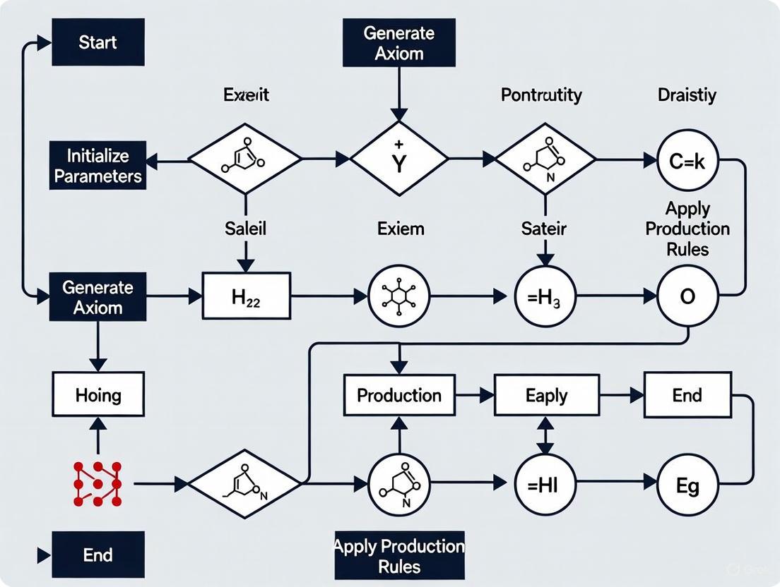
The following diagram illustrates the complete workflow for L-system implementation, from core components through biological interpretation:

Production Rule Application Mechanism

The following diagram details the parallel rewriting mechanism that distinguishes L-systems from other formal grammars:

The Scientist's Toolkit: Research Reagent Solutions

Table 4: Essential Computational Tools for L-System Research

Tool/Component	Function	Research Application	Example Implementation
Symbolic Processing Engine	Applies production rules in parallel	Core L-system iteration	Python dictionary mapping: {'A':'AB', 'B':'A'} [7]
Turtle Graphics Interpreter	Visualizes geometric meaning of symbols	Spatial representation of development	F: forward draw, +: turn left, -: turn right, [/]: stack branching [6]
Parameter Optimization Framework	Adjusts angles, lengths, and rule probabilities	Fine-tuning biological realism	Evolutionary algorithms for parameter optimization
Context-Sensitive Parser	Handles neighborhood-dependent rules	Modeling cell-cell interactions in development	Pattern matching with left/right context symbols
Stochastic Rule Selector	Chooses rules probabilistically	Introducing phenotypic variation	Weighted random selection based on probability values

Advanced Applications in Plant Development Modeling

Contemporary research has expanded L-system applications to integrate physiological and environmental factors. Recent approaches adapt natural tree growth mechanisms through hierarchical subdivision of design domains, utilizing principal stress lines extracted from feature regions to create structurally efficient tree-like architectures [8]. This methodology enables the generation of free-form tree-like structures through superimposition of mechanical patterns and iterative form evolution, with the final morphology representing the outward expression of internal forces [8].

Such advanced implementations demonstrate how L-systems have evolved from purely descriptive models to generative frameworks that balance aesthetic requirements with structural performance, offering new approaches for creating architectural alternatives with asymmetric, curvilinear forms without compromising structural integrity [8].

Formal grammars provide a structured framework for modeling the complex growth patterns found in biological systems, particularly in plant development. Among these, Lindenmayer systems (L-systems) stand as a specialized class of parallel rewriting systems developed specifically to model multicellular organism development [1] [9]. Unlike Chomsky grammars designed for linguistic analysis, L-systems employ parallel application of production rules to simulate the simultaneous growth processes characteristic of biological development [1]. This parallelism fundamentally distinguishes L-systems from traditional formal grammars and makes them particularly suitable for simulating biological processes where multiple cell divisions occur concurrently.

The integration of formal grammar classes—context-free, context-sensitive, and deterministic L-systems—provides researchers with a hierarchical modeling framework capable of capturing biological phenomena at varying complexity levels. Context-free grammars offer simplicity and computational efficiency, context-sensitive grammars enable modeling of environmental interactions, and deterministic L-systems provide the foundation for procedural generation of plant structures with predictable developmental sequences [1] [10] [11]. This grammatical hierarchy serves as the theoretical underpinning for algorithmic simulation of plant development in computational botany and bio-inspired procedural generation.

Theoretical Foundations and Comparative Analysis

Formal Definitions and Properties

Deterministic, Context-Free L-Systems (D0L-systems) are defined by the tuple G = (V, ω, P), where V is an alphabet of symbols, ω is the axiom (initial string), and P is a finite set of productions or rewriting rules [1] [11]. In a D0L-system, rules take the form A → x, where A ∈ V is a single symbol and x is a string over V, with exactly one rule for each symbol in V [11]. The derivation proceeds in parallel, with all symbols in the string being rewritten simultaneously in each derivation step [1].

Context-Free Grammars in the Chomsky hierarchy are defined by the quadruple G = (N, Σ, P, S), where N is a set of nonterminal symbols, Σ is a set of terminal symbols, P is a set of production rules, and S is the start symbol [10]. Rules are of the form A → γ, where A is a single nonterminal and γ is a string of terminals and nonterminals. Critically, these rules apply individually rather than in parallel, and the replacement of symbols is not sensitive to their context [10].

Context-Sensitive Grammars (CSG) are formally defined with rules of the form αAβ → αγβ, where A is a nonterminal, α and β are strings of symbols that form the context, and γ is a non-empty string [10]. This context dependence allows the replacement of A by γ only when it appears between α and β. An equivalent definition requires that for every production u → v, the length of u is less than or equal to the length of v (non-contracting grammar) [10].

Comparative Analysis of Grammar Classes

Table 1: Comparative Analysis of Formal Grammar Classes in Biological Modeling

Feature	Context-Free Grammars	Deterministic L-Systems (D0L)	Context-Sensitive Grammars
Rule Application	Sequential	Parallel	Sequential
Biological Interpretation	Limited due to sequential nature	Ideal for simultaneous cell divisions	Suitable for context-dependent development
Computational Complexity	Polynomial time parsing	Linear time generation	Exponential time complexity
Representational Power	Limited to non-interactive structures	Self-similar fractals, plant-like forms	Cross-serial dependencies, interactive growth
Example Applications	Syntax parsing in linguistics	Algae growth, fractal trees, simple plants	aⁿbⁿcⁿ patterns, complex dependencies

Hierarchical Relationships and Expressive Power

The relationship between these grammar classes follows a well-defined hierarchy of expressive power. Context-free grammars are strictly less powerful than both context-sensitive grammars and L-systems due to their lack of context sensitivity and parallel application respectively [10]. While L-systems and context-sensitive grammars are not directly comparable—as they operate on different principles (parallel vs. sequential application)—both exceed the representational capacity of context-free grammars for biological modeling [1] [10].

This hierarchy has significant implications for plant development modeling. The famous language {aⁿbⁿcⁿ | n ≥ 1}, which represents coordinated growth of three cell types in specific proportions, cannot be generated by context-free grammars but can be generated by context-sensitive grammars [10]. Similarly, L-systems can generate developmental sequences with self-similar properties that context-free grammars cannot capture [1] [11].

D0L-Systems: Protocols for Plant Morphogenesis

Experimental Protocol: Inference of D0L-Systems from Developmental Sequences

Objective: Automatically infer the deterministic context-free L-system (D0L-system) from a sequence of strings representing developmental stages of plant structures.

Materials and Reagents:

• Input Data: Developmental sequence of strings (ω₁, ω₂, ..., ωₙ) obtained through image segmentation of temporal plant growth data [11]
• Software Tools: Plant Model Inference Tool for Deterministic Context-Free L-systems (PMIT-D0L) [11]
• Computational Resources: Standard workstation for L-systems with ≤31 symbols; high-performance computing for systems with >100 symbols

Procedure:

• Data Preprocessing: Convert input image sequence to developmental strings using segmentation algorithms [11]
• Search Space Reduction: Apply mathematical constraints to limit possible productions based on length requirements and symbol mappings
• Encoding Scheme Selection: Implement length-based encoding to search through allowable combinations of production lengths
• Genetic Algorithm Execution:
  • Initialize population of candidate L-systems
  • Evaluate fitness based on match to developmental sequence
  • Apply selection, crossover, and mutation operators
  • Iterate until convergence or stopping criteria met
• Validation: Verify inferred L-system reproduces full developmental sequence

Troubleshooting:

• For inaccurate inferences: Increase population size or generations in genetic algorithm
• For slow convergence: Implement novel length-based encoding schemes [11]
• For ambiguous results: Incorporate additional developmental stages as input

Case Study: Algae Growth Modeling

Lindenmayer's original L-system for algae growth demonstrates the fundamental principles of D0L-systems [1]:

• Variables: A, B
• Axiom: A
• Rules: (A → AB), (B → A)

This simple system produces the developmental sequence: n=0: A, n=1: AB, n=2: ABA, n=3: ABAAB, n=4: ABAABABA, which exhibits the Fibonacci property in the lengths of the strings [1]. The sequential application of these rules mimics the cell division patterns in algal filaments.

Figure 1: D0L-System Derivation for Algae Growth

Research Reagent Solutions for L-System Implementation

Table 2: Essential Research Tools for L-System Experiments

Tool/Reagent	Function	Application Example
VLab (Virtual Laboratory)	L-system visualization and simulation	3D plant growth rendering [11]
PMIT-D0L	Automated inference of L-systems from data	Reverse-engineering plant development [11]
Genetic Algorithm Framework	Search mechanism for rule inference	Optimizing L-system parameters [11]
Image Segmentation Pipeline	Conversion of plant images to symbolic strings	Preprocessing temporal growth data [11]
Turtle Graphics Renderer	Geometric interpretation of L-system strings	Converting symbolic strings to plant structures [1]

Context-Sensitive Grammars: Protocols for Environmental Interaction

Experimental Protocol: Context-Sensitive Modeling of Plant-Environment Interactions

Objective: Develop context-sensitive grammar rules to model how environmental factors influence plant development.

Materials:

• Formal Grammar Framework: Context-sensitive grammar implementation platform
• Environmental Data: Soil composition, light gradients, mechanical pressure metrics
• Plant Response Metrics: Growth rates, branching angles, biomass allocation

Procedure:

• Context Identification: Determine which environmental factors serve as contextual triggers in production rules
• Rule Formulation: Create context-sensitive productions of the form αAβ → αγβ where α and β represent environmental conditions
• Validation Testing: Verify rules generate appropriate structures under specified environmental contexts
• Parameter Optimization: Adjust rule parameters to match empirical growth data

Sample Rule Design: For shade-avoidance response in competitive environments:

This context-sensitive rule triggers stem elongation when a plant segment (A) detects low sunlight conditions.

Case Study: Coordinated Growth Pattern Generation

The canonical example of context-sensitive power in biological modeling is the generation of the language {aⁿbⁿcⁿ | n ≥ 1}, representing three interdependent cell types growing in coordination [10]. The grammar for this language requires context-sensitive rules that allow symbols to be replaced based on their context:

• S → aBC | aSBC
• CB → CZ
• CZ → WZ
• WZ → WC
• WC → BC
• aB → ab
• bB → bb
• bC → bc
• cC → cc

This grammar demonstrates how context sensitivity enables maintenance of proportional relationships during development, similar to morphogen gradients in plant development [10].

Figure 2: Context-Sensitive Grammar Derivation Process

Integration and Advanced Applications

Hybrid Approach: Combining Grammar Classes for Multiscale Modeling

Modern plant development modeling often requires integrating multiple grammar classes to capture different aspects of growth:

• D0L-systems model the overall architectural development
• Context-sensitive rules incorporate environmental responses
• Parametric extensions add continuous parameters for quantitative traits

Protocol for Hybrid Model Development:

• Architectural Foundation: Establish base topology using D0L-systems
• Environmental Integration: Add context-sensitive rules for abiotic factors
• Parameter Optimization: Tune continuous parameters using measurement data
• Validation: Compare model output to empirical growth series

Emerging Techniques: Quantum and Graph-Based Approaches

Recent advances in L-system inference include graph-based classical and quantum approaches to deterministic L-system inference [12]. These methods:

• Translate L-system inference to maximum independent set problems
• Utilize quantum algorithms for enhanced search capabilities
• Characterize string sequences as graphs to identify production rules
• Offer potential polynomial-time solutions for certain inference problems

The characteristic graph of a sequence of strings enables reformulation of the inference problem into computationally tractable forms, potentially accelerating the automated discovery of L-systems from experimental data [12].

The integration of formal grammar classes—context-free, context-sensitive, and deterministic L-systems—provides a powerful framework for modeling plant development algorithms. D0L-systems offer efficient generation of self-similar structures characteristic of plant morphology, while context-sensitive grammars enable the modeling of environmental interactions and coordinated growth patterns. The ongoing development of automated inference tools like PMIT-D0L represents a significant advancement toward reducing the manual effort required to construct accurate plant models. As these techniques mature, integrating graph-based and quantum approaches may further accelerate our ability to reverse-engineer the algorithmic principles underlying plant development, with profound implications for computational botany, agricultural optimization, and bio-inspired engineering.

Computational modeling has become an indispensable tool in developmental biology, providing a framework to integrate complex processes across spatial and temporal scales. Among these approaches, Lindenmayer systems (L-systems) stand as a foundational pillar in theoretical biology for modeling multicellular development and plant morphogenesis [5]. Originally conceived by Aristid Lindenmayer in 1968, L-systems are parallel rewriting systems that excel at capturing the recursive, branching patterns ubiquitous in biological structures [5] [13]. This protocol details the methodology for interpreting these abstract string-based models into visual structures using turtle graphics, thereby bridging the gap between formal language theory and observable biological form. The ability to generate complex structures from simple rules makes L-systems particularly valuable for modeling plant root development and other branching architectures, where intricate patterns emerge from local cellular interactions [13].

Core Concepts and Definitions

L-System Fundamentals

An L-system is defined formally as a tuple G = (V, ω, P), where:

• V (the alphabet) is a set of symbols containing both constants and variables
• ω (the axiom) is the initial string of symbols from V
• P is a set of production rules defining how each symbol is rewritten

The power of L-systems lies in their parallel rewriting capability; unlike Chomsky grammars where rules are applied sequentially, L-systems rewrite all symbols in the string simultaneously during each derivation step. This parallel application makes them particularly suited for modeling biological development where cell divisions occur concurrently [5].

Turtle Graphics Interpretation

Turtle graphics provides a geometrical interpretation method for L-system strings. The "turtle" is a virtual drawing agent with a state defined by its position (x, y) and orientation θ in 2D or 3D space. Symbols in the final L-system string command the turtle's movement and drawing actions [14] [15].

Table: Core Turtle Graphics Commands and Their Biological Analogues

Symbol	Turtle Action	Biological Analogue	Parameters
F	Move forward, drawing a line	Cell elongation or growth	Step length d
f	Move forward without drawing	Internal growth without structural change	Step length d
+	Turn left (counterclockwise)	Differential growth causing left curvature	Angle δ
-	Turn right (clockwise)	Differential growth causing right curvature	Angle δ
[	Push current state onto stack	Branch initiation point	None
]	Pop state from stack	Return to main axis after branching	None

Materials and Research Reagent Solutions

Table: Essential Computational Tools for L-system Research

Research Tool	Function/Purpose	Implementation Examples
L-system Interpreter	Executes rewriting rules and manages derivation	Racket #lang lindenmayer [15], Lindenmayer (Python)
Turtle Graphics Renderer	Visualizes interpreted strings as geometrical structures	lindenmayer/turtle, lindenmayer/3d-turtle libraries [15]
Parameter Optimization Algorithms	Finds parameter values that match biological structures	Genetic algorithms, particle swarm optimization [14]
Sensitivity Analysis Tools	Tests model robustness to parameter variations	Monte Carlo sampling, Sobol sequence analysis [13]

Protocol: Interpreting L-Systems with Turtle Graphics

L-System Definition and Setup

Objective: Define the L-system grammar that captures the developmental rules of the biological structure of interest.

• Identify Biological Axiom: Determine the initial structure (ω) analogous to the biological starting state (e.g., a single root apical meristem cell) [13].
• Define Alphabet (V): Establish symbols representing biological states or actions:
  • Variables: Symbols that are rewritten (e.g., X, A, B representing undifferentiated cell types)
  • Constants: Symbols that remain fixed (e.g., F, +, -, [, ] representing structural actions)
• Formulate Production Rules (P): Create rules that mimic developmental processes. For example:
  • X → F[+X]F[-X]+X captures apical growth with lateral branching [15]
  • F → FF represents exponential cell proliferation

Turtle Graphics Parameterization

Objective: Establish the mapping between L-system symbols and graphical actions.

• Set Initial Turtle State: Initialize position (typically (0,0)) and orientation (typically 0° or 90°).
• Define Step Size: Establish the distance d corresponding to one 'F' command, representing a biological length unit (e.g., cell length).
• Set Turning Angle: Define the angle δ for '+' and '-' commands, capturing growth direction changes.
• Configure Stack: Implement the push ('[') and pop (']') mechanism for managing branching points, analogous to saving/restoring developmental states.

Implementation and Execution

Objective: Execute the L-system and render the geometrical structure.

• String Derivation: Iteratively apply production rules to the axiom for n generations:

• String Interpretation: Parse the final string and execute corresponding turtle commands:
  • For each symbol, call the associated function with current turtle state and variables [15]
  • Maintain a stack for branch point preservation
• Rendering: Generate the visual representation from the turtle's path.

Worked Example: Simulating a Simple Branching Structure

Biological Context: Modeling the development of a plant root system with alternating lateral branches [13].

• L-system Definition:

  • Alphabet V: {X, F, +, -, [, ]}
  • Axiom ω: X
  • Production rules P: X → F[+X]F[-X]+X F → FF
  • Angle δ = 20°
  • Iterations: n = 7

• Implementation Code Framework:

  This produces a branching structure similar to developmental patterns observed in root systems [15].

Advanced Applications in Plant Development Research

Integrating Biological Mechanisms

Contemporary L-system models extend beyond simple branching to incorporate specific biological mechanisms:

• Auxin Transport Models: Incorporate PIN-FORMED auxin efflux carriers to simulate phyllotaxis and venation patterning [13]
• Gene Regulatory Networks: Embed Boolean network models into L-system symbols to simulate cell fate determination
• Mechanical Feedback: Implement feedback between tissue mechanics and cell growth rates

Table: Quantitative Parameters for Biological L-system Models

Biological Process	L-system Representation	Key Parameters	Typical Values
Root branching periodicity	Symbol rewriting interval	Branching angle	45-90°
Phyllotaxis	Angular increment at apex	Golden angle	137.5°
Vascular patterning	Context-sensitive rules	Auxin threshold	0.1-1.0 nM
Apical dominance	Inhibition propagation	Inhibition range	3-5 internodes

Model Validation and Robustness Testing

Objective: Ensure the L-system model produces biologically plausible patterns across parameter variations.

• Sensitivity Analysis: Systematically vary parameters (angles, step sizes, recursion depth) and quantify output differences.
• Robustness Testing: Verify that qualitative patterns persist across parameter ranges, reflecting biological stability [13].
• Experimental Comparison: Compare generated structures with microscopic imaging of actual biological specimens.

Troubleshooting and Optimization

Common Implementation Challenges

• Unrealistic Branching Density: Adjust production rule probabilities or introduce suppression mechanisms analogous to apical dominance
• Geometrical Artifacts: Ensure turtle state (position, orientation) is properly saved/restored at branch points
• Exponential Complexity: Limit recursion depth (n) or implement pruning rules for biologically irrelevant structures

Performance Considerations

For models with high complexity (>10 iterations) or extensive parameter exploration:

• Implement efficient string rewriting algorithms
• Utilize GPU acceleration for turtle graphics rendering
• Employ optimization algorithms (e.g., genetic algorithms) for parameter fitting to experimental data [14]

The integration of L-systems with turtle graphics provides a powerful methodology for modeling biological development from simple rules to complex structures. This protocol establishes a foundation for researchers to implement these techniques in studying plant development, with particular relevance to root architecture, vascular patterning, and branching morphogenesis. The approach enables hypothesis testing about developmental mechanisms through in silico experimentation, complementing wet-lab approaches in developmental biology. Future directions include integrating L-systems with physiological models and environmental response mechanisms to create more comprehensive models of plant development.

L-systems, or Lindenmayer systems, are a type of formal grammar and parallel rewriting system introduced in 1968 by the theoretical biologist and botanist Aristid Lindenmayer [1]. Originally devised to describe the behavior of plant cells and model the growth processes of simple multicellular organisms, L-systems provide a mathematical framework for simulating biological development [5] [1]. The core components of an L-system are an alphabet of symbols, a set of production rules that expand each symbol into a larger string of symbols, an initial axiom string from which construction begins, and a mechanism for translating generated strings into geometric structures [1]. This formalism has proven exceptionally well-suited for modeling the branching patterns and fractal architectures ubiquitous in nature, from microscopic bacteria to macroscopic trees and vascular systems.

Key Biological Applications and Case Studies

Modeling Plant Development and Architecture

The formalism of L-systems has emerged as a major paradigm for constructing Functional–Structural Plant Models (FSPMs) [4] [16]. In these models, a plant is represented by a bracketed string where elements, called modules, represent the plant’s components such as internodes, meristems, and flowers [4]. A set of rules then defines how each module transforms over time, simulating the plant's development. For example, a simple L-system for algae growth can generate a sequence of Fibonacci words, mirroring a fundamental growth pattern found in nature [1]. Modern implementations, such as L-Py, leverage dynamic programming languages like Python to create complex and modular plant models without the syntactic overhead of statically-typed languages, thus making the technology more accessible to biologists [4] [16].

Simulating Arterial Branching Patterns

Parametric L-systems have been formulated to generate branching tree structures that incorporate the physiological laws of arterial branching [17]. These generated trees are, by construction, fractal structures. With appropriate parameter choices, they can exhibit branching patterns observed in arterial trees, particularly those with a preponderant value of the asymmetry ratio. Key physiological parameters that can be incorporated include the asymmetry ratio, the area ratio, branch diameters, and branching angles [17]. The basic L-system model for a symmetrical tree structure consisting of repeated bifurcations uses graphical commands to represent lines, branching points, and directional turns, providing a language that carries directly from botanical to arterial structures [17].

Computational Modeling of Plant Root Development

Computational models, including those based on L-systems, are uniquely suited to integrate processes like gene expression, cell-cell signaling, and cell growth across wide temporal and spatial scales to investigate plant root development [13]. These are mechanistic models, whose purpose is to obtain an understanding of the underlying biological mechanisms rather than merely describing reality or predicting the future in quantitative detail [13]. A key principle in building such models is to incorporate the right level of detail; increased complexity comes at the cost of reduced ease of understanding. Therefore, models should be kept as simple as possible while still capturing the essential processes needed to reproduce the phenomenon of interest [13].

Table: Key Parameters for Biological L-system Models

Application Area	Key Model Parameters	Biological Counterpart	Representation
Plant Architecture [4]	Age (e.g., of an apex), Internode length & radius, Maximum age	Plant components (metamers, meristems), Growth limits	Modules: Apex(age), Internode(length, radius)
Arterial Branching [17]	Asymmetry ratio, Area ratio, Branch diameters, Branching angles	Vessel size and bifurcation geometry	Fractal tree structures with physiological constraints
Stochastic Growth [18]	Generation (g), Random segment length, Random angle	Natural variation and plasticity in form	Parametric modules with random functions (e.g., randbetween)

Experimental Protocols and Methodologies

Protocol: Modeling a Simple Branching Structure using L-Py

This protocol outlines the steps to create a basic plant branching model using the L-Py framework, which integrates L-systems into the Python language [4] [16].

• Module Declaration: Begin by declaring the modules that will represent the plant's components. Modules can have parameters to characterize their state.

  In this code, Apex and Internode are declared as modules with their respective parameters [4].

• Define Constants and Axiom: Set global constants and define the axiom, which is the initial string from which development begins.

  The axiom is a single Apex module with an initial age of zero [4].

• Specify Production Rules: Write the rules that govern the development of each module over discrete time steps.

  • The Internode rule gradually increases its radius by dr at each step [4].
  • The Apex rule checks if the maximum age has not been reached. If not, it produces an internode, a branching structure (enclosed in brackets), and a new apex. The symbols /(137.5) and +(40) control the orientation of new growth, simulating phyllotaxis or branching angles [4] [16].

• Execution and Visualization: Run the L-Py interpreter to execute the L-system for a specified number of steps. The resulting string can be interpreted graphically using turtle graphics to visualize the plant structure in 3D [4].

Protocol: Generating a Fractal Tree with Branching

This methodology details the creation of a fractal binary tree, a classic example that demonstrates the generation of complex, self-similar structures from simple rules [1].

• System Definition: Define the core components of the L-system.

  • Variables: 0, 1
  • Constants: "[", "]"
  • Axiom: 0
  • Rules: (1 → 11), (0 → 1[0]0) [1]

• Iterative Rewriting: Apply the production rules in parallel for a set number of iterations (n).

  • n = 0: 0
  • n = 1: 1[0]0
  • n = 2: 11[1[0]0]1[0]0
  • n = 3: 1111[11[1[0]0]1[0]0]11[1[0]0]1[0]0 [1]

• Turtle Graphics Interpretation: Translate the generated string into a geometric structure by assigning graphical commands to each symbol.

  • 0: Draw a line segment ending in a leaf.
  • 1: Draw a line segment.
  • [: Push the current position and angle onto a stack, then turn left 45 degrees.
  • ]: Pop the position and angle from the stack, effectively moving the turtle back to the last branch point, then turn right 45 degrees [1]. The push and pop operations, facilitated by the square brackets, are crucial for managing branching points and creating a hierarchical, tree-like structure.

Protocol: Incorporating Randomization and Parameters

To model natural variability, L-systems can be extended to parametric and stochastic forms [18]. This protocol describes how to introduce randomness to create more organic and less rigid artificial structures.

• Define Parametric Modules: Use modules with parameters that can change over time or across instances. Example: L(g) represents a module with a generation parameter g [18].

• Create Parametric Rules: Write production rules that use these parameters to control growth. Example: L(g) → [rf(2-g/2)L(g+1)][lf(2-g/2)L(g+1)] [18]. This rule creates an H-tree structure where the segment length decreases as the generation g increases.

• Introduce Stochasticity: Replace fixed parameters with random functions within specified ranges to mimic natural variation. Example: Instead of a fixed angle, use rot("randbetween(-20-5, -20+5)") to introduce slight variations in branching angles [18]. Example: Use fwd("randbetween(100/(g+1)-10, 100/(g+1)+10)") to vary segment lengths randomly around a mean value that decreases with generation [18].

Diagram 1: Core workflow for developing an L-system model, from definition to visualization.

The Scientist's Toolkit: Research Reagent Solutions

Table: Essential Components for L-system Based Modeling

Tool / Component	Function / Role in Modeling	Example Implementation / Notes
L-Py Framework [4] [16]	An L-system simulation environment embedded in Python.	Enables high-level programming, model reusability, and avoids compilation overhead. Ideal for rapid prototyping and teaching.
Formal Grammar Interpreter (e.g., cpfg, lpfg) [4]	The core engine that executes the parallel rewriting rules of the L-system.	Earlier implementations were often based on static languages (C++, Java) for high computational efficiency.
Turtle Graphics System [1] [18]	Translates the symbolic string generated by the L-system into a geometric structure.	Symbols are interpreted as commands for a virtual "turtle" (e.g., move forward, turn). Essential for visualization.
MTG (Multiscale Tree Graph) Data Structure [4]	Represents plant architecture at multiple scales of organization.	Allows for seamless integration of L-systems with a wide spectrum of pre-existing plant analysis tools.
Parametric & Stochastic Modules [18]	Introduces variability and context-dependent growth into models.	Uses parameters (e.g., generation, length) and random functions to create more natural, non-identical structures.

Diagram 2: Architecture of a typical L-system modeling framework, showing core components.

Implementing Virtual Botany: From Theory to Functional-Structural Plant Models

Functional–structural plant models (FSPMs) have emerged as a powerful family of computational approaches that use 3D representations of plant architecture to simulate physiological and ecophysiological processes [16]. Among these, Lindenmayer systems (L-systems) have established themselves as a major paradigm for modeling plant development, originating from Aristid Lindenmayer's work in 1968 as a formalism for describing developmental processes in biology [16]. The inherent recursive nature of plant structures makes L-systems particularly well-suited for simulating plant architecture, where plants are represented by bracketed strings of modules representing components like metamers, meristems, and other organs [16].

Modern L-system research has progressed beyond context-free string-rewriting systems to incorporate three advanced paradigms: parametric, stochastic, and environmentally-sensitive approaches. Parametric L-systems associate numerical parameters with symbols, enabling the representation of continuous variations in plant structures. Stochastic L-systems incorporate probabilistic production rules to capture the natural variability observed in plant development. Environmentally-sensitive L-systems respond to external factors such as light, water, and physical obstacles, creating dynamic feedback between plants and their environment [19]. These advanced paradigms have transformed L-systems from purely descriptive tools into predictive frameworks capable of simulating complex plant-environment interactions with high biological fidelity.

Parametric L-Systems: Encoding Continuous Variation

Core Principles and Implementation

Parametric L-systems extend the basic formalism by associating parameters with symbols in the L-system alphabet. This enables the representation of continuous characteristics such as internode length, leaf area, branch radius, and physiological age. In parametric L-systems, each module consists of a symbolic name and an optional set of parameters that can be manipulated according to mathematical expressions within production rules [16].

The L-Py implementation exemplifies modern parametric L-system frameworks, embedding L-system constructs within the Python programming environment. This integration provides a simplified syntax through dynamic typing while maintaining expressive power. A basic parametric L-system structure in L-Py includes module declarations, constants, an initial axiom, and production rules that govern development [16] [4].

Table 1: Key Components of Parametric L-Systems in L-Py

Component	Syntax Example	Function
Module Declaration	module Apex(age), Internode(length, radius)	Defines module types and their parameters
Constants	MAX_AGE, dr = 10, 0.02	Sets fixed values used in productions
Axiom	Apex(0)	Defines the initial state of the system
Production Rules	Apex(age): if age<MAX_AGE: produce Internode(1,0.05)/(137.5)[+(40)Apex(age+1)] Apex(age+1)	Specifies how modules transform over time

Application Notes: Simulating Architectural Development

Parametric L-systems effectively simulate the architectural models defined by Hallé et al., which categorize plant development patterns based on combinations of a small number of botanical characters such as branching type, flowering, and axis differentiation [20]. The 23 identified architectural models, each named after a botanist (e.g., the Corner model for unbranched plants like palms, the Rauh model for rhythmic growth patterns like pines), can be encoded using parametric L-systems by adjusting key growth parameters [20].

The physiological age parameter is particularly significant in this context, as it describes the differentiation patterns of shoots and branches along physiological gradients [20]. By organizing development according to physiological age, complex structures can be simulated with a limited number of parameters, making parametric L-systems both computationally efficient and botanically accurate.

Stochastic L-Systems: Modeling Natural Variability

Theoretical Foundations

Stochastic L-systems incorporate variability into plant development by assigning probabilities to production rules, capturing the inherent randomness observed in natural systems. Unlike deterministic models that produce identical outputs from the same initial conditions, stochastic L-systems generate populations of plants with individual variations while maintaining species-specific characteristics [20].

The mathematical analysis of stochastic L-systems often employs generating functions and multitype branching processes to characterize probability distributions and moments of organ numbers in plant structures [21]. By modeling plant architectural development as a combination of subprocesses driving bud population dynamics—branching and differentiation—researchers can compute generating functions for the entire system by compounding the associated generating functions [21]. For differentiation processes, multivariate phase-type random vectors provide a novel framework for analysis [21].

Analytical Methods and Moment Computation

The GreenLab model exemplifies the application of stochastic L-systems in functional-structural plant modeling. As one of the few FSPMs that can be calibrated mathematically, GreenLab simulates the 23 botanical architectural models using parameters derived from physiological age concepts [20]. The model couples an architectural component with sink-source functions of individual organs, formalizing organogenesis, photosynthesis, and morphogenesis processes [20].

For stochastic versions of GreenLab (GL2), theoretical computation of mean and variance of organ numbers and biomass production provides fast and accurate prediction of model outputs without time-consuming Monte Carlo simulations. Moments of organ numbers are obtained by applying compound rules from probability generating functions (PGFs) combined with substructure decomposition [20]. The following experimental protocol outlines the methodology for implementing and analyzing stochastic L-systems:

Protocol 1: Implementing Stochastic L-Systems for Plant Development Analysis

• Define Stochastic Parameters: Identify key developmental processes to model stochastically, such as bud fate (death, rest, or creation of metamers), branch emergence, or organ size variation. Assign probabilities to these events based on empirical observations.

• Architectural Model Setup: Configure the plant architectural model according to botanical principles, specifying physiological ages of meristems and their differentiation patterns. For tree species following the Rauh model, implement rhythmic growth with probabilistic branching.

• Generate Function Computation: Apply compound rules from probability generating functions to determine moments of organ numbers. Use substructure decomposition to handle complex branching patterns.

• Biomass Production Modeling: Compute biomass production at each growth cycle using differential statistics. The recurrent function for biomass production (Qn) at plant age n can be expressed as: Qn = En × Σ[i=1 to ta] (Nn-i+1L × Σ[j=1 to i] pL(j) × Qn-(i-j)-1 / Dn-(i-j)) / (α + β × Σ[j=1 to i] pL(j) × Qn-(i-j)-1 / Dn-(i-j)) where En is environmental factor, Nn-i+1L is leaf count, pL is leaf biomass sink, and Dn is demand function [20].

• Moment Calculation: Compute covariance matrices between numbers of metamers and biomass production using inductive approaches at each growth cycle.

• Validation: Compare theoretical moment computations with empirical measurements from real plants or simulated populations to validate model accuracy.

Figure 1: Stochastic L-System Analysis Workflow

Environmentally-Sensitive L-Systems: Integrating Feedback

Dynamic Plant-Environment Interactions

Environmentally-sensitive L-systems represent the most advanced paradigm, incorporating feedback between plant development and environmental factors such as light, water, wind, and temperature [19]. These systems move beyond predetermined growth patterns to create dynamic responses where plant architecture emerges from continuous interaction with its surroundings.

Research in computational vegetation modeling has demonstrated how environmentally-sensitive L-systems can simulate both developmental responses (long-term structural adaptations) and immediate physical responses to environmental stimuli [19]. For example, tree responses to long-term and short-term wind influence can be captured, showing how developmental models adapt growth patterns while physical models simulate branch movement [19]. Similarly, plastic tree models can respond to light availability or obstacles, redistributing growth toward optimal light conditions [19].

Application Notes: Source-Sink Modeling and Resource Allocation

The GreenLab model implements environmental sensitivity through source-sink relationships, where biomass production depends on photosynthetic capacity (source) and organ demands (sink) [20]. Environmental factors are incorporated through the En parameter in the biomass production equation, representing growth potential modified by local conditions [20]. This approach has been applied to various agricultural and horticultural crops, including cotton, maize, chrysanthemum, and apple trees [20] [19].

For apple trees specifically, researchers have developed source-sink developmental models that simulate water consumption, photosynthesis, and resulting fruit production [19]. These models have been extended to study the effects of pruning, with optimization algorithms determining which branches should be removed to maximize light interception [19].

Table 2: Environmental Factors and Their Implementation in L-Systems

Environmental Factor	Model Implementation	Plant Response
Light Availability	Photosynthetic module with spatial light competition	Phototropic growth, branch orientation, leaf positioning
Wind	Mechanical stress simulation on branching structure	Thicker trunks, reduced height, directional growth
Water Availability	Soil water module with root uptake dynamics	Reduced leaf area, altered biomass partitioning
Temperature	Thermal time accumulation (degree-days)	Phenological development rate, growth cycle timing
Obstacles	Collision detection and avoidance algorithms	Directional growth alteration, crown asymmetry

Experimental Protocols and Validation Frameworks

Protocol for 3D Plant Reconstruction and Inverse Modeling

Recent advances in machine learning have enabled the reconstruction of parametric plant representations from 3D scan data, creating digital twins of real plants that can be used in simulation scenarios [22]. The following protocol outlines this approach:

Protocol 2: 3D Plant Reconstruction via Inverse Procedural Modeling

• Data Acquisition: Capture 3D point clouds of target plants using photogrammetry (Structure from Motion) or LiDAR scanning. For optimal results, acquire multiple overlapping images from different angles (minimum 24 positions) around the plant [23].

• Preprocessing: Clean point cloud data by removing noise, outliers, and non-plant elements. Align and register multiple scans into a unified coordinate system.

• Synthetic Dataset Generation: Create a training dataset using L-system-based procedural models to generate virtual plants with known parameters. Apply simulated acquisition noise and occlusions to bridge the gap between synthetic and real data [22].

• Network Architecture: Implement a recursive neural network trained on the synthetic dataset. Exploit the binary tree structure of plant architecture using a recursive auto-encoder to learn latent representations of plant geometry and branching structure [22].

• Parameter Inference: For a given input point cloud, use the trained network to infer the parametric representation (L-string) that best approximates the observed plant architecture.

• Validation: Compare reconstructed models with actual plants using geometric metrics (leaf area, branch angles) and topological measures (branching patterns). For strawberry plants, validation against manual measurements of petiole length and leaf size has shown strong agreement (AdjR² = 0.78 for leaf area) [23].

Protocol for Radiative Transfer Image Simulation

The integration of L-systems with radiative transfer models enables the simulation of remote sensing imagery with realistic plant canopies:

Protocol 3: Radiative Transfer Image Simulation of Synthetic Canopies

• Canopy Generation: Use L-systems to simulate plant canopies at specific growth stages, incorporating empirical measurements of leaf size, petiole length, and branching patterns [23].

• Geometric Parameter Extraction: From simulated canopies, extract key structural information including leaf area index, leaf angle distribution, and canopy height profiles [23].

• Spectral Characterization: Measure spectral properties (reflectance and transmittance) of plant components (leaves, stems) and background elements (soil, mulch) using field spectroradiometers [23].

• Radiative Transfer Modeling: Use Discrete Anisotropic Radiative Transfer (DART) software or similar tools to simulate sensor-reaching radiation based on canopy geometry, component spectral properties, and acquisition parameters (sun position, viewing geometry, sensor characteristics) [23].

• Vegetation Index Analysis: Extract spectral vegetation indices (e.g., NDVI, SRre) from simulated imagery and develop regression models to predict biophysical parameters (leaf area, dry biomass) [23].

• Validation: Compare simulated images with actual remote sensing data, and validate biophysical parameter predictions against field measurements.

Figure 2: Radiative Transfer Simulation Workflow

Table 3: Research Reagent Solutions for Advanced L-System Modeling

Tool/Resource	Function	Application Context
L-Py	L-system implementation in Python dynamic language	Plant architecture simulation, educational modeling [16]
GreenLab	Mathematical FSPM with sink-source functions	Biomass production, organ size prediction, agricultural applications [20]
GreenScilab	Scilab-based toolbox for plant simulation	Parameter estimation from measurements, plant visualization [20]
OpenAlea	Open-source platform for plant modeling	Complex model integration, modular FSPM development [16]
DART	Discrete Anisotropic Radiative Transfer model	Simulating remote sensing imagery from 3D canopy models [23]
MTG (Multi-Scale Tree Graph)	Data structure for plant representation	Managing plant description at multiple scales of organization [16]
Recursive Neural Networks	Deep learning for plant structure analysis	Inverse procedural modeling, parameter estimation from point clouds [22]

Future Directions and Research Opportunities

The integration of advanced L-system paradigms with emerging technologies presents numerous research opportunities. Deep neural models that encode tree structures as latent spaces show promise for both reconstruction and novel plant generation [19]. The Rhizomorph project exemplifies next-generation approaches that model the coordinated function of shoots and roots, creating more comprehensive virtual plant representations [19].

Validation remains a challenge in computational plant modeling, with perceptual models like ICTree representing innovative approaches for assessing the realism of synthetic plants through large-scale user evaluation and AI-based quality prediction [19]. As these technologies mature, digital twins of plants will become increasingly important for agricultural planning, climate change impact assessment, and fundamental plant research.

The Crops in Silico initiative highlights the growing importance of multiscale computational models for agricultural applications, connecting genetic traits with phenotypic expression through in silico experimentation [19]. These approaches enable researchers to explore "what-if" scenarios virtually, accelerating the development of improved crop varieties and management practices.

Advanced L-system paradigms have transformed plant modeling from a descriptive tool to a predictive science, enabling researchers to simulate plant development with unprecedented biological fidelity. As these approaches continue to integrate with machine learning and high-performance computing, they will play an increasingly vital role in addressing global challenges in food security and environmental sustainability.

Functional–structural plant models (FSPMs) combine 3D representations of plant architecture with simulations of physiological processes to study plant development [16] [4]. L-systems, a formal grammar system introduced by Aristid Lindenmayer in 1968, have emerged as a major paradigm for constructing these models [5] [1]. Several programming frameworks have implemented L-systems, primarily extending general-purpose programming languages. This application note provides a detailed comparative analysis of three prominent implementations: L-Py (Python), L+C (C++), and XL (Java), within the context of plant development algorithms research.

Core Framework Characteristics

Table 1: Fundamental Framework Characteristics

Characteristic	L-Py	L+C	XL
Host Language	Python [16] [24]	C++ [16] [4]	Java [25] [4]
Typing System	Dynamic [16] [4]	Static [16] [4]	Static [25] [4]
Syntax Complexity	Simple, intuitive [16]	Complex, requires expertise [16]	Moderate, Java-based [25]
Learning Curve	Shallow [16] [4]	Steep [16] [4]	Moderate [25]
Execution Model	Interpreted [16]	Compiled [16]	Compiled/Portable [4]
License	CeCILL (GPL-compatible) [24]	Not specified	Open-source [25]

Technical Implementation Specifications

Table 2: Technical Implementation Details

Technical Aspect	L-Py	L+C	XL
Modular Representation	L-strings with MTG integration [16] [4]	Parametric modules [16]	Graph-based structures [4]
ODE Support	Python scientific libraries	Custom implementations [25]	Built-in rate assignment operator [25]
Platform Support	Cross-platform (Python) [24]	Platform-dependent [16]	Cross-platform (Java) [4]
Integration Capabilities	OpenAlea ecosystem [16] [24]	Limited external integration	GroIMP platform [25]
3D Visualization	Integrated environment [24] [26]	External tools required	Built-in GroIMP visualization [25]

Framework Architecture and Relationships

Experimental Protocols and Methodologies

Protocol 1: Basic Plant Growth Simulation

Objective: Implement a simple branching structure to compare syntax and development approaches across frameworks.

L-Py Implementation:

Source: Adapted from Frontiers in Plant Science [16]

L+C Implementation Notes:

• Requires type declarations for all parameters
• Compilation step necessary before execution
• C++ syntax for control structures [16] [4]

XL Implementation Notes:

• Java-based type system
• Integrated in GroIMP platform
• Graph-based structure representation [25]

Validation Metrics:

• Branching pattern accuracy
• Parameter consistency across growth stages
• 3D geometry generation

Protocol 2: Differential L-Systems with ODE Integration

Objective: Model physiological processes using differential equations within L-system framework.

XL Implementation:

Source: ScienceDirect [25]

Numerical Integration Methods:

• Forward Euler (basic, stability issues)
• Crank-Nicolson (implicit, better stability)
• Adaptive step-size Runge-Kutta (high accuracy) [25]

Experimental Parameters:

• Step size sensitivity (0.01-1.0 time units)
• Stability thresholds
• Computational performance metrics

Protocol 3: Multiscale Plant Representation

Objective: Integrate organ-level and cellular-level processes using MTG data structures.

L-Py Specific Protocol:

• Import MTG data structure from OpenAlea
• Define scale-specific production rules
• Implement between-scale communication protocols
• Validate topological consistency [16]

Validation Framework:

• Scale transition accuracy
• Data structure integrity
• Memory usage profiling

The Scientist's Toolkit

Table 3: Essential Research Reagent Solutions

Tool/Component	Framework	Function	Implementation Notes
MTG Data Structure	L-Py	Multiscale plant representation	Pre-integrated in OpenAlea [16]
ODE Solver Library	XL	Differential equation integration	Built-in rate assignment operator [25]
Geometry Primitives	All	3D structure generation	Framework-specific implementations
Ray Tracing Engine	L+C, XL	Light interaction simulation	L-PEACH model extension [25]
Optimization Tools	L-Py	Parameter calibration	Integrated development environment [24]
Stochastic Rule Engine	All	Probabilistic growth patterns	Varies by framework implementation

Research Application Workflow

Performance Considerations and Best Practices

Computational Efficiency

• L+C offers superior execution speed for large-scale simulations due to C++ optimization and static typing [16] [4]
• L-Py provides faster development cycles and interactive debugging at the cost of runtime performance [16]
• XL balances performance and portability through Java virtual machine optimization [25]

Model Development Guidelines

• For teaching and prototyping: L-Py's simple syntax and immediate feedback facilitate rapid iteration [16]
• For production-scale models: L+C's performance advantages justify the steeper learning curve [16]
• For physiological process modeling: XL's integrated ODE framework provides numerical stability [25]

Validation Framework

• Cross-framework consistency checking
• Numerical stability analysis for ODE integration
• Morphological validation against empirical data
• Sensitivity analysis for parameter optimization

The selection of an L-system framework depends on research priorities: L-Py excels in accessibility and rapid prototyping, L+C provides maximum computational performance, and XL offers robust differential equation integration within a portable Java environment. Understanding these tradeoffs enables researchers to align computational tools with specific plant development modeling requirements.

The formalism of L-systems has emerged as a major paradigm for constructing Functional–Structural Plant Models (FSPMs), which use 3D representations of plant architecture to simulate physiological and ecophysiological processes [16] [4]. These computational models require sophisticated software frameworks that balance development efficiency with runtime performance. This application note explores the computational trade-offs between static and dynamic typing within L-Py, an L-system simulation framework embedded in Python, focusing on its implications for rapid biological modeling in plant development research.

L-Py represents a significant evolution in L-system implementations by adapting the formalism to Python, a dynamic language [16]. Previous L-system implementations like L+C and XL were based on statically-typed languages (C++ and Java, respectively), which require explicit variable type definitions and involve more syntactic overhead [4]. The core innovation of L-Py lies in its integration of L-systems with Python's dynamic typing system, creating a modeling environment that prioritizes rapid prototyping and flexibility while maintaining computational capabilities for complex biological simulations.

Theoretical Foundations: Typing Systems in Computational Modeling

Fundamental Differences Between Static and Dynamic Typing

The distinction between static and dynamic typing represents a fundamental dichotomy in programming language design with direct implications for scientific modeling:

• Static Typing: Variable types are explicitly declared and verified at compile-time, before program execution [27] [28]. This approach enables comprehensive error checking and performance optimizations during compilation.
• Dynamic Typing: Variable types are determined implicitly at runtime based on assigned values [27] [28]. This eliminates the need for explicit type declarations, offering greater flexibility and faster prototyping capabilities.

In the context of L-system implementations for plant modeling, this distinction translates to significant differences in development workflow, error detection, and computational performance [16] [4].

Historical Context of L-System Implementations

The development of L-system frameworks has evolved through several generations of typing system implementations:

Table: Evolution of L-System Frameworks and Their Typing Systems

Framework	Base Language	Typing System	Primary Advantages
cpfg	Dedicated language	Static	Mathematical notation foundation [4]
L+C (lpfg)	C++ extension	Static	High performance, complex FSPM support [16] [4]
XL	Java extension	Static	Portability, object-oriented structures [4]
L-Py	Python extension	Dynamic	Simple syntax, rapid prototyping, high reusability [16] [4]

L-Py Framework Architecture and Dynamic Typing Implementation

Core Components of L-Py

L-Py integrates L-system constructs directly into Python's syntax while maintaining compatibility with established L-system conventions [16] [4]. The framework's core architectural components include:

Figure 1: L-Py integrates L-system constructs with Python and multiscale plant representation.

Module System

Plant structures are decomposed into physical units called modules, consisting of a symbolic name and optional parameters [16]. Modules with the same name represent identical component types (e.g., Internode, Apex). In L-Py, module parameters are Python objects that can be of any type without explicit declaration [16] [4].

Axiom Definition

The initial state of the simulation is defined by a specific string of modules called the axiom, declared using the Axiom keyword [16]. This represents the starting structure from which plant development simulations proceed.

Production Rules

Developmental processes are encoded through production rules that define how modules transform over time [16]. These rules are declared using the production keyword and determine how each module produces new modules, enabling the simulation of growth and branching patterns.

L-Py Syntax Example with Dynamic Typing

The following code illustrates how L-Py leverages Python's dynamic typing for concise model specification:

This example demonstrates key advantages of dynamic typing in L-Py [16] [4]:

• No type declarations required for module parameters (age, l, r)
• Variables (MAX_AGE, dr) can be assigned without explicit typing
• Conditional logic uses standard Python syntax without type constraints
• The produce statement generates new modules with dynamically typed parameters

Computational Trade-offs: Quantitative Analysis

Performance and Development Efficiency Metrics

The choice between static and dynamic typing involves inherent trade-offs between computational performance and development efficiency. For biological modeling applications, these trade-offs must be evaluated in the context of specific research requirements.

Table: Performance and Development Characteristics of Typing Systems in Plant Modeling

Characteristic	Static Typing (L+C/XL)	Dynamic Typing (L-Py)
Type Checking	Compile-time [27] [28]	Runtime [27] [28]
Development Speed (Initial)	Slower due to type declarations [27]	Faster prototyping [16] [27]
Error Detection	Early in development cycle [27] [28]	May appear during execution [27] [28]
Runtime Performance	Optimized by compiler [27] [28]	Interpretation overhead [16] [27]
Code Refactoring	Strong IDE support [27]	Manual and riskier [27]
Learning Curve	Steeper [16] [4]	More shallow [16] [4]

Implementation Efficiency in Biological Modeling

Research comparing typing system efficiency reveals nuanced trade-offs for scientific applications. Ousterhout [16] notes that a typical statement in a dynamic language equals 100-1000 machine instructions, compared to 1-10 instructions for static languages. This abstraction level enables higher-level programming constructs but incurs runtime performance costs.

For L-system implementations specifically, L-Py's dynamic typing provides distinct advantages for model exploration and iteration [16]:

• Rapid prototyping of novel plant architectures
• Flexible integration of diverse data structures and algorithms
• Simplified syntax reduces barriers for biologists with limited programming experience
• Seamless interoperability with Python's scientific ecosystem (NumPy, SciPy, matplotlib)

Experimental Protocols for Typing System Evaluation in Plant Modeling

Protocol 1: Comparative Model Development Efficiency

Objective: Quantify the development time and code complexity differences between static and dynamic typing approaches for implementing a standard FSPM.

Materials:

• L-Py framework (dynamic typing)
• L+C or XL framework (static typing)
• Standardized plant model specification (e.g., sunflower phyllotaxis)

Methodology:

• Implement the reference model in both frameworks
• Record development time for initial implementation
• Measure lines of code (LOC) and cyclomatic complexity
• Implement three sequential model modifications
• Record time required for each modification
• Document any type-related errors encountered

Expected Outcomes: L-Py should demonstrate significantly faster initial implementation and modification times, with potentially higher runtime performance for the statically-typed implementation.

Protocol 2: Runtime Performance Benchmarking

Objective: Evaluate computational performance differences for complex canopy development simulations.

Materials:

• L-Py installation with standard benchmarking suite
• Equivalent L+C implementation of benchmark models
• Controlled computational environment

Methodology:

• Execute growth simulations for 100, 1000, and 10,000 developmental steps
• Measure memory utilization at each scale
• Record execution time for each simulation
• Profile specific operations (module production, parameter calculation, geometric computation)
• Compare results across frameworks

Expected Outcomes: Statically-typed implementations will likely demonstrate superior performance at large scales, while L-Py may show advantages for smaller-scale exploratory simulations.

Protocol 3: Multiscale Model Integration

Objective: Assess the flexibility of each typing system for integrating models across biological scales.

Materials:

• L-Py with MTG (Multiscale Tree Graph) integration capabilities
• Reference implementation in statically-typed framework
• Multiscale dataset (molecular, cellular, organ, plant)

Methodology:

• Implement cross-scale signaling pathways (e.g., hormone transport)
• Integrate molecular-scale data with organ-level development
• Measure code complexity for multiscale interactions
• Evaluate model extensibility for adding new biological scales

Expected Outcomes: L-Py's dynamic typing should demonstrate superior flexibility for integrating heterogeneous data types across biological scales.

The Scientist's Toolkit: Essential Research Reagents for L-Py Modeling

Table: Core Components for L-Py Experimental Workflows

Component	Function	Implementation in L-Py
MTG Data Structure	Represents plant topology at multiple scales [16] [4]	Integrated into L-Py, enables multiscale analysis
L-system Interpreter	Executes production rules to simulate development [29]	Embedded in Python with dynamic typing
Geometric Primitives	Defines 3D structure of plant components [16]	High-level description at different scales
Parameter Estimation Tools	Optimizes model parameters from experimental data [29]	Integrated development environment with optimization
Visualization System	Renders 3D plant architecture for analysis [29]	Interactive visualization of simulation results

Application Notes for Research Scenarios

Scenario 1: Rapid Hypothesis Testing in Plant Development

For research requiring rapid iteration on developmental hypotheses, L-Py's dynamic typing provides significant advantages. The simplified syntax and lack of compilation overhead enable researchers to quickly implement, test, and modify theoretical models [16].

Recommended Workflow:

• Implement core developmental hypothesis as L-Py production rules
• Use Python's dynamic typing for flexible parameter adjustment
• Visually validate simulation results against experimental data
• Iteratively refine model rules based on validation
• Formalize validated model with comprehensive testing

Scenario 2: Large-Scale Canopy Simulation

For large-scale simulations requiring optimal performance, the trade-offs favor static typing approaches. However, L-Py can still be effective through strategic implementation:

Optimization Strategies:

• Use Python's profiling tools to identify computational bottlenecks
• Implement performance-critical components as compiled extensions
• Leverage L-Py's integration with high-performance computing resources
• Employ hybrid approaches with dynamic typing for control logic and static typing for core computations

Figure 2: Iterative modeling workflow leveraging L-Py for rapid prototyping.

The computational trade-offs between static and dynamic typing in L-system implementations reflect broader tensions in scientific computing between development agility and runtime performance. L-Py's dynamic typing approach offers compelling advantages for rapid biological modeling, particularly during exploratory research phases where flexibility and rapid iteration are prioritized.

For plant development researchers, L-Py represents an optimal solution for hypothesis-driven model development, educational applications, and exploratory algorithm design [16]. The framework's integration with Python's scientific ecosystem and its simplified syntax significantly lower barriers to entry while maintaining capabilities for sophisticated simulations. As biological modeling increasingly requires integration across scales and data types, dynamic typing systems like that implemented in L-Py provide the flexibility necessary for cutting-edge research in functional-structural plant modeling.

Functional–structural plant models (FSPMs) are computational tools that simulate the growth and development of plants in three dimensions (3D), explicitly representing the architecture of a plant as a network of elementary units while simultaneously modeling the physiological processes that drive its development [30]. These models have emerged as a powerful paradigm for integrating our understanding of plant form and function [31]. A key mathematical formalism underpinning many FSPMs is the L-system, a string rewriting system that effectively captures the recursive, branching nature of plant topology [32]. This case study details the systematic construction of an FSPM, from its foundational axioms to a mature, validated model, framed within the context of advanced L-systems research for plant development algorithms.

Foundations of FSPM Development

Core Concepts and Definitions

The development of an FSPM is motivated by the need to understand the integration of plant form and function and their interaction with the environment [30]. Unlike more abstract plant models that use simplified representations, a fundamental feature of FSPMs is the explicit representation of plant structure as a collection of elementary units, such as metamers, internodes, and buds [30] [31]. This explicit architectural representation enables the modeling of how local physiological processes and environmental interactions give rise to global plant structure and behavior.

A primary challenge in FSPM development is managing model uncertainty. Two key categories of uncertainty are:

• Non-uniqueness: The existence of alternative, equally valid representations for model components with no a priori way to decide between them [33].
• Incomplete specification: The characteristic that a model may explain some, but not all, observed features of a system [33]. The FSPM construction process is inherently progressive, with uncertainty being reduced as the model is iteratively improved and assessed against an increasing number of criteria [33].

The Role of L-Systems in FSPMs

L-systems provide a critical mathematical foundation for many FSPMs. They consist of an alphabet of symbols, production rules for rewriting strings, and an initial axiom, enabling the generation of complex, branching structures through iterative string rewriting [32]. This formalism is particularly suited for modeling plant morphogenesis because it naturally captures the recursive and modular nature of plant development. Within an FSPM framework, L-systems are often extended and integrated with other modeling techniques to simulate not only topology but also the biomechanical and physiological processes that influence growth [30] [31].

Methodological Framework: The Pareto Optimal Assessment Cycle

A robust methodology for developing and assessing FSPMs is the Pareto Optimal Assessment Cycle (POMAC), which uses multi-criteria evaluation and evolutionary computation to quantify and reduce model uncertainty [33]. The workflow for this method is as follows:

Stage 1: Initial Model Definition

The first stage involves establishing the core components of the modeling framework.

• Model Objectives and Scope: Clearly define the biological theory or system the FSPM is designed to investigate. For example, a model might aim to explain the pattern of foliage reiteration on old-growth branches [33] or the partitioning of carbon within a tree canopy [30].
• Parameter and Range Definition: Identify all model parameters and define the biologically feasible ranges within which their values can be sought during the calibration process. This includes morphological parameters (e.g., phyllotactic angles, internode elongation rates) and physiological parameters (e.g., photosynthetic efficiency, carbon allocation coefficients) [33].
• Assessment Criteria Definition: Establish multiple, quantifiable criteria for evaluating model performance. These criteria should be selected to test specific aspects of the theory and are categorized as follows [33]:
  • Quantitative Domain Tests: Based on empirical data (e.g., total height, number of branches, leaf area index).
  • Explicit Prediction Tests: Assess features the model is explicitly designed to predict.
  • Structural Formulation Tests: Evaluate between alternative structures or functions in the model.

Table 1: Example Assessment Criteria for a Branch Reiteration FSPM (based on BRANCHPRO model from [33])

Criterion Category	Specific Variable	Acceptable Range	Data Source
Quantitative Domain	Total number of reiterated shoots	15 - 25	Field measurements
Explicit Prediction	Spatial distribution pattern of shoots	Matches observed clustering index	3D digitized data
Structural Formulation	Annual biomass production	±10% of independent estimate	Allometric equations

Stage 2: Evolutionary Computation

This stage involves an automated search for parameter sets that best satisfy the multiple assessment criteria.

• Algorithm Initialization: An initial population of model parameterizations (e.g., 100 individuals) is created with random values within the predefined ranges [33].
• Multi-Criteria Evaluation: Each parameterization in the population is run, and its performance against all assessment criteria is calculated [33].
• Pareto Ranking and Selection: Parameterizations are ranked based on Pareto dominance. A solution is "non-dominated" if it is better than all others in at least one criterion. The highest-ranked, non-dominated individuals are selected [33].
• Breeding and Iteration: A new generation is created by "breeding" the selected individuals through genetic operators like crossover (exchange of parameter values) and mutation (small random changes). This process repeats for many generations (e.g., 500) until a stable Pareto Frontier is achieved [33].

Stage 3: Pareto Set Analysis

The final set of non-dominated solutions (the Pareto Optimal Set) is analyzed to inform model development.

• Analyzing Set Structure: The number of distinct non-dominated groups in the Pareto Set reveals model uncertainty. A single, tight cluster of parameterizations indicates low uncertainty, while multiple, disparate groups suggest the model cannot simultaneously satisfy all criteria well, pointing to structural issues [33].
• Model Refinement: The analysis identifies deficiencies in the model's mathematical structure or component functions. For instance, if the Pareto analysis reveals a fundamental trade-off between simulating height growth and branch number, it may indicate a missing feedback mechanism in the model that couples apical and lateral growth [33]. This insight drives iterative refinement of the model.

Experimental Protocol: Multi-Criteria Assessment of an FSPM

This protocol provides a detailed methodology for implementing the POMAC framework.

Pre-Modeling Setup

• Empirical Data Collection: Gather high-quality 3D architectural data. This can be achieved using magnetic, sonic, or laser digitizers to capture the explicit geometry and topology of the study plants [30]. Extract key metrics for assessment criteria.
• Computational Environment: Select and set up an appropriate modeling platform that supports L-systems and integrated physiological functions, such as OpenAlea [31] or GroIMP [30].
• Parameter Range Justification: Define parameter bounds based on literature reviews and preliminary experimental data to ensure the evolutionary algorithm explores a realistic parameter space.

Execution of Evolutionary Computation

• Algorithm Configuration:
  • Population size: 100 individuals.
  • Number of generations: 500.
  • Mutation rate: 1% per parameter.
  • Crossover rate: 80%.
• Fitness Evaluation Scripting: Implement a script that automatically runs the FSPM for a given parameter set, extracts the simulated outputs corresponding to the assessment criteria, and calculates the performance metrics (e.g., absolute difference from measured values).
• Parallel Computing: Distribute the evaluation of the population across multiple computing cores or nodes to reduce total computation time.

Post-Simulation Analysis

• Pareto Frontier Visualization: Generate pairwise plots of all assessment criteria, highlighting the non-dominated solutions to visualize the trade-offs between different model objectives.
• Parameter Sensitivity Analysis: Analyze the distribution of parameter values within the Pareto Optimal Set. Parameters with a narrow, unimodal distribution are well-constrained by the data, while those with wide or multimodal distributions contribute significantly to model uncertainty [33].
• Model Output Validation: Use the Pareto-optimal parameter sets to run the final model and compare its predictions against a reserved subset of validation data not used during the calibration process.

The Scientist's Toolkit: Essential Research Reagents and Materials

The development and application of FSPMs rely on a suite of specialized tools and software platforms.

Table 2: Key Research Reagent Solutions for FSPM Development

Tool/Platform Name	Type	Primary Function in FSPM Research
L-system based Platforms (e.g., GroIMP, L-studio)	Software Framework	Provides a formal language and environment for implementing plant growth rules using L-system grammars and generating 3D visualizations [30] [32].
OpenAlea	Modeling Platform	Facilitates the assembly of modular FSPM components from various sources and the analysis of simulation results [30] [31].
Multi-Scale Tree Graph (MTG)	Data Structure	Offers a generic and unified way to represent and analyze plant architecture at multiple scales of organization [30].
3D Laser Scanner / Digitizer	Measurement Hardware	Captures the explicit 3D geometry of real plants for model parameterization, assessment, and validation [30].
Evolutionary Computation Algorithm	Optimization Software	Automates the search for parameter values that achieve multiple assessment criteria, enabling the calculation of the Pareto Optimal Set [33].
Color Contrast Analyzer (CCA)	Accessibility Tool	Ensures that all diagrams, user interfaces, and visual outputs associated with the FSPM meet WCAG guidelines for color contrast, aiding usability for all researchers [34] [35].

Visualization and Communication

Effective communication of FSPM structure and results is critical. The following diagram outlines the core logical relationships in an FSPM, from environmental input to architectural output.

Furthermore, adhering to accessibility standards in all visual outputs is a hallmark of professional scientific communication. The following color contrast standards, derived from WCAG guidelines, must be followed for all diagrams, charts, and user interfaces [36] [35].

Table 3: WCAG Color Contrast Requirements for Scientific Visualizations

Visual Element Type	WCAG Level AA Minimum Ratio	WCAG Level AAA Minimum Ratio	Practical Application
Normal Text	4.5:1	7:1	Labels, legends, and text within diagrams.
Large Text (18px+ or 14px+ Bold)	3:1	4.5:1	Section headers and titles in figures.
Graphical Objects & UI Components	3:1	-	Lines, arrows, and symbols against their background.

Constructing a mature FSPM is a rigorous, iterative process that moves from a basic axiom or conceptual model to a sophisticated tool capable of explaining complex plant phenomena. By grounding the model in L-systems and adopting a structured methodology like the Pareto Optimal Assessment Cycle, researchers can systematically quantify and reduce model uncertainty. The integration of multi-criteria assessment, evolutionary computation, and rigorous visualization standards ensures that the resulting FSPM is not only a powerful predictive tool but also a robust platform for testing hypotheses about the fundamental principles governing plant development and its interaction with the environment. This structured approach from axiom to maturity is essential for advancing the field and generating reliable, actionable insights in plant science.

Application Note: Conceptual Framework and Quantitative Foundations

This document provides detailed application notes and protocols for integrating L-system models with Multiscale Tree Graph (MTG) data structures, a cornerstone for developing functional–structural plant models (FSPMs) within advanced plant development algorithms research. This integration is designed to capture the complex multiscale nature of plant architecture, from organ-level geometry to whole-plant topology.

The formalism of L-systems has emerged as a major paradigm for constructing FSPMs [16] [4]. In L-systems, a plant is represented by a bracketed string of modules, where each module represents a plant component (e.g., an internode, meristem, or leaf) [16]. A set of production rules then defines how each module transforms over time, simulating development. Meanwhile, the MTG formalism provides a common way to represent plants at several scales of organization [16]. The integration of these two in the L-Py framework allows for a seamless connection between the dynamic, rule-based simulation of L-systems and the multiscale analytical capabilities of MTGs [16].

Table 1: Core Quantitative Parameters for Multi-Scale Plant Architecture Modeling

Model Component	Scale	Key Quantitative Descriptors	Data Type	Typical L-Py Module Example
Internode	Organ	Length (mm), Radius (mm), Volume (mm³)	Continuous	Internode(length, radius) [16]
Apex/Meristem	Organ	Age (phytomers), Development Stage (e.g., vegetative/generative)	Discrete, Categorical	Apex(age) [16]
Branching System	Topology	Branching Angle (degrees), Phyllotactic Angle (degrees), Number of Branches	Continuous, Discrete	/(137.5)[+(40)Apex(age+1)] [16]
Plant Topology	Whole-Plant	Graph-based measures (Connectivity, Centrality), Topology [37]	Graph	Embedded MTG Data Structure [16]
Plant Geometry	Whole-Plant	Surface Area (m²), Volume (m³), Spatial Coordinates (x,y,z) [37]	Continuous	L-string 3D Interpretation [16]

Table 2: Research Reagent Solutions for Computational Modeling

Item Name	Function/Description	Application in Protocol
L-Py Simulation Environment	An L-system framework embedded in the dynamic Python language, enabling high-level programming and integration with MTG data structures [16].	Core platform for writing, executing, and visualizing L-system models that are natively linked to MTGs.
OpenAlea Platform	An open-source platform for plant modeling; the distribution point for the L-Py software and related components [16].	Provides the ecosystem and libraries necessary for building complex, multi-component models.
MTG Data Structure	A formal graph-based structure to represent the multiscale topology and geometry of plants [16].	Serves as the underlying data model for representing the simulated plant architecture across scales.
Python Language	A powerful, dynamic programming language that simplifies model development and enables scripting and integration [16].	The base language for L-Py, used to define model logic, control flow, and data analysis.

Protocol: Implementing an Integrated L-System and MTG Model

This protocol details the steps to create a functional–structural plant model using the L-Py framework, wherein the simulated plant architecture is represented as an MTG. The model will simulate the development of a simple plant with branching topology, capturing its growth dynamics at multiple scales.

Equipment and Software

• Computer with a standard operating system (Windows, macOS, or Linux)
• OpenAlea platform installation (includes L-Py)
• A standard text editor or integrated development environment (IDE)

Detailed Procedure

Step 1: Module and Axiom Definition

Declare the plant components as L-system modules with their key parameters. Define the initial state of the plant (the axiom).

• In an L-Py file, declare the modules using the module keyword.
• Define the axiom using the Axiom keyword to specify the starting point of the simulation, typically a meristem or apex.

L-Py Code Implementation:

Step 2: Production Rule Specification

Formulate the set of context-free production rules that govern the development of each module over discrete time steps.

• Initiate rule declarations with the production: keyword.
• For an Apex module, check if its age is below a predefined MAX_AGE.
• If true, use the produce keyword to generate new modules: an Internode, a turtle geometry command for phyllotactic angle, and two new Apex modules (one for continued growth and one for a new branch).
• Define a rule for the Internode module to simulate radial growth over time.

L-Py Code Implementation:

Step 3: Model Execution and MTG Coupling

Run the L-system simulation within the L-Py environment. The resulting plant structure is automatically compiled into an MTG data structure, enabling multiscale analysis.

• Execute the L-Py script.
• The interpreter applies the production rules iteratively to the axiom for a predefined number of steps.
• At each step, the L-string is updated, and the corresponding MTG is maintained, capturing the plant's topology and geometry.
• The final MTG can be exported or analyzed directly using MTG-specific tools available in the OpenAlea ecosystem.

Step 4: Data Extraction and Analysis

Query the generated MTG to extract quantitative descriptors of plant morphology and topology at different scales.

• Use MTG traversal functions to access plant components.
• Extract geometrical descriptors (e.g., total length, volume) and topological descriptors (e.g., number of branches, branching order) for analysis.
• The integrated framework allows for the seamless passing of information between the L-system simulation and the MTG representation, facilitating complex analyses.

Visualization of the Multi-Scale Modeling Logic

The following diagram, generated from the provided DOT script, illustrates the logical workflow and data flow between the core components of the integrated modeling system.

Expected Outcomes and Interpretation

• Primary Outcome: A dynamic, growing 3D model of a branching plant structure.
• Data Analysis: The integrated MTG allows researchers to quantify key architectural traits. For example, analyzing the distribution of Internode lengths and radii can provide insights into resource allocation, while topological analysis of the graph can reveal patterns in branching complexity.
• Troubleshooting: Common issues include L-system rules that do not fire as expected, often due to module naming or parameter mismatches. Ensure module declarations exactly match their use in the axiom and productions. For MTG analysis, verify the scale at which specific traits are being measured.

Computational Botany in Practice: Solving Implementation Challenges and Enhancing Realism

This document outlines common pitfalls encountered in the development of L-systems for modeling plant development and provides detailed application notes and experimental protocols to address them. L-systems, or Lindenmayer systems, are a mathematical formalism used to model the growth and development of plants through iterative rule applications [38] [16]. While powerful for generating complex, organic structures from simple rules, practical implementation often confronts three critical challenges: geometric artifacts from imprecise turtle graphics, computational complexity in branching structures, and performance bottlenecks in large-scale rendering [39]. This guide is structured to provide researchers with actionable methodologies for diagnosing and resolving these issues, framed within the context of plant development algorithm research.

Pitfall 1: Geometric Artifacts in Turtle Graphics Interpretation

Nature of the Problem

Geometric artifacts—such as visible gaps between connected segments, unrealistic overlaps, and inconsistent scaling—commonly arise during the interpretation of L-strings into 3D geometry (a process known as "topologizing") [39]. These artifacts stem from inconsistencies in the state management of the virtual "turtle" that translates symbolic strings into geometric models. Imperfect handling of the turtle's position, orientation, and the scaling of sequential parts can break the visual continuity of structures like stems and branches, compromising biological accuracy.

Experimental Protocol: Quantifying and Correcting Artifacts

Objective: To systematically identify the sources of geometric artifacts and validate correction methods. Materials: L-system interpreter, 3D rendering environment, a defined L-system grammar (e.g., for a tree trunk).

• Model Generation: Implement a production rule set for a branching structure. For example:
  • Axiom: T
  • Rules: T=FFF[/+TX][////+TX]/////////+TX and X=F[/+FX][////+FX]/////////+FX [39].
• Turtle State Logging: Instrument the interpreter to log the turtle's full state (location, forward rotation, up rotation, and current radius) before and after the interpretation of each symbol (e.g., F, [, ], +, -) across multiple iterations.
• Artifact Identification: Render the generated mesh and visually inspect for gaps and overlaps. Correlate artifact locations with the logged state data to identify erroneous state transitions (e.g., incorrect position after a pop operation from ]).
• Correction Implementation: Implement and test the following corrective measures:
  • State Stack Fidelity: Ensure the push ([) and pop (]) operations perfectly save and restore the entire turtle state, including orientation vectors and current radius.
  • Conical Frustum Connection: When drawing a segment for F, generate a conical frustum whose top cap is oriented to match the turtle's new position and orientation after the move, ensuring a seamless connection to the subsequent segment [39].
• Validation: Re-render the model and verify the elimination of artifacts. Quantify improvement by measuring the reduction in visible gaps/overlaps.

Table 1: Common Geometric Artifacts and Solutions

Artifact Type	Root Cause	Corrective Action
Gaps between segments	Top cap orientation not matching subsequent segment's base.	Model segments as conical frustums with configurable top orientation [39].
Branch misalignment	Inconsistent state restoration upon popping from the stack with ].	Ensure the state stack manages location, orientation, and radius faithfully.
Unnatural tapering	Constant radius usage throughout the L-string.	Apply a RadiusFactor (e.g., 0.7) to the turtle's radius when initiating new branches [39].

Visualization: Turtle State Workflow

The following diagram illustrates the critical state transitions of the turtle during L-string interpretation, highlighting points where artifacts can originate.

Diagram 1: Turtle state interpretation workflow.

Pitfall 2: Branching Recursion Complexity

Nature of the Problem

L-systems excel at modeling branching structures, but this requires managing branching recursion, where a single parent module spawns multiple child modules [40]. This presents a dual challenge: Conceptual Abstraction, where models fail to infer the correct recursive generative rules from visual examples, and Computational Explosion, where the number of modules grows exponentially with each iteration, leading to memory overflow and performance degradation [40] [39]. Current multimodal AI systems show a striking failure rate in this area, with less than 2% success in generating correct code for tree fractals, underscoring its fundamental difficulty [40].

Experimental Protocol: Benchmarking Branching Complexity

Objective: To evaluate an L-system implementation's robustness in handling deep recursion and complex branching. Materials: L-system interpreter, memory profiling tools, a set of L-system grammars with increasing branching factor (e.g., binary, ternary).

• Grammar Definition: Define a parameterized branching L-system.
  • Axiom: A
  • Rule: A=F[+A][-A] (binary branching) or A=F[+A][-A][&A] (ternary branching).
  • Configure AngleDegrees and MoveDistance [39].
• Controlled Iteration: Generate models for iterations (n) 1 through 10. Record the length of the final L-string and the total memory consumed by the interpreter for each n.
• Performance Profiling: Use profiling tools to track:
  • Peak memory usage during L-string expansion.
  • Time spent on string rewriting versus geometric interpretation.
• Complexity Analysis: Plot L-string length and memory usage against the number of iterations n. The curve should reveal exponential growth, confirming the computational complexity.
• Mitigation Strategy: Implement and test a depth-limiting mechanism that halts recursion after a predefined number of steps or when the turtle's radius falls below a visually perceptible threshold.

Table 2: Branching Complexity Analysis

Iteration (n)	Branching Factor	Theoretical L-string Length	Measured Memory Usage (MB)
3	2	31	~1.2
5	2	511	~5.5
7	2	8,191	~65.0
3	3	121	~2.1
5	3	9,841	~95.0

Visualization: Branching Recursion Complexity

The diagram below maps the workflow for diagnosing and mitigating issues related to branching complexity.

Diagram 2: Branching complexity diagnosis and mitigation.

Pitfall 3: Performance Bottlenecks in Rendering

Nature of the Problem

High-fidelity L-system models can contain millions of triangles for trunks and branches, compounded by orders of magnitude more instanced leaves, leading to severe performance bottlenecks during rendering [39]. The primary issues are CPU-GPU Data Transfer, where issuing individual draw calls for numerous small objects (like leaves) is prohibitively slow, and Vertex Processing Overload, where the GPU is overburdened with processing a massive number of vertices, especially in shadow passes [39]. These bottlenecks manifest as low frame rates and long rendering times, hindering interactive visualization and experimentation.

Experimental Protocol: Profiling and Optimizing Rendering

Objective: To identify rendering performance bottlenecks and quantify the improvement from optimization techniques. Materials: A complex L-system model (e.g., a tree with >100k triangles), real-time rendering API (e.g., DirectX, OpenGL), GPU profiling tool (e.g., Nsight Graphics).

• Baseline Establishment: Render the model in a controlled scene. Use profiling tools to capture key metrics:
  • Frame time (ms).
  • Number of draw calls.
  • GPU time spent in vertex shaders.
  • Time spent in shadow passes.
• Bottleneck Identification: Analyze the profile.
  • A high number of draw calls for similar objects (leaves) indicates a CPU bottleneck.
  • High vertex shader load indicates a GPU geometry processing bottleneck [39].
• Optimization Implementation:
  • Geometry Instancing: For repetitive objects like leaves, replace individual draw calls with a single instanced draw call. Pass per-instance data (transformation matrices, sub-UV coordinates) via a StructuredBuffer [39].
  • Level of Detail (LOD): Implement a distance-based LOD system that renders simplified versions of complex models when they are far from the camera.
  • Culling: Employ view-frustum culling to avoid processing geometry outside the visible screen area.
• Validation: Re-profile the application after applying optimizations. Compare the same metrics against the baseline to measure performance gain.

Table 3: Performance Bottleneck Analysis and Solutions

Bottleneck Category	Key Symptom	Optimization Strategy	Expected Outcome
CPU / Draw Calls	High number of DrawIndexed calls for leaves.	Implement geometry instancing via a single DrawIndexedInstanced call [39].	Drastic reduction in CPU submission overhead.
GPU / Vertex Processing	Long scoreboard stalls in vertex shader; high vertex count.	Use LOD and culling to reduce the total vertices processed per frame.	Improved GPU vertex throughput and shorter frame times.
GPU / Shadow Pass	Shadow pass takes nearly as long as the main pass [39].	Apply simplified meshes or LODs for shadow rendering.	Significant reduction in overall frame rendering time.

Visualization: Performance Optimization Workflow

This diagram outlines the systematic process of diagnosing and addressing rendering performance bottlenecks.

Diagram 3: Performance bottleneck diagnosis workflow.

The Scientist's Toolkit: Research Reagent Solutions

Table 4: Essential Software and Tools for L-system Research

Tool / Reagent	Type	Primary Function	Application Note
L-Py [16]	Modeling Framework	An L-system simulation framework embedded in Python.	Enables high-level programming, model reusability, and avoids compilation overhead. Ideal for rapid prototyping in plant development research.
MinimalTurtle [40]	Interpretation Interface	A minimal graphics interface (move, turn, pen up/down).	Isolates visual-to-symbolic rule abstraction, preventing models from bypassing mathematical reasoning via library recall. Useful for benchmarking.
GPU Profiler (e.g., Nsight) [39]	Diagnostic Tool	Provides a detailed breakdown of GPU resource usage and performance bottlenecks.	Critical for identifying vertex shader stalls and optimizing rendering of complex plant models.
Geometry Instancing [39]	Rendering Technique	Submits multiple copies of a mesh (e.g., leaves) in a single draw call.	Dramatically reduces CPU overhead. Implementation involves a StructuredBuffer for per-instance data like transformation matrices.
Depth-Limiting & Tapering	Modeling Technique	Halts recursion at a set depth and scales branch radius per iteration.	Manages computational explosion and creates more realistic, visually tapering plant structures.

The formalism of L-systems, introduced by Aristid Lindenmayer in 1968, provides a powerful framework for simulating the development of biological organisms, particularly plants [5] [1]. While basic L-system models can generate complex, self-similar structures, creating biologically realistic simulations requires the integration of advanced techniques that capture the inherent variability, coordinated growth, and adaptive responses observed in living systems. This application note details protocols for incorporating stochastic variation, allometric relationships, and plastic growth into L-system models, framed within a broader research thesis on advancing plant development algorithms. Designed for researchers and computational biologists, these methodologies aim to bridge the gap between abstract mathematical models and the nuanced reality of plant growth, with potential applications in computational botany, agricultural technology, and digital twin development for plants.

Technical Background

L-System Fundamentals

An L-system is a parallel rewriting system defined as a formal grammar ( G = (V, \omega, P) ), where:

• ( V ) is the alphabet of symbols (variables and constants).
• ( \omega ) (the axiom) is the initial string of symbols from ( V ).
• ( P ) is a set of production rules that define how each symbol is replaced by a string of successor symbols [1].

The recursive application of these rules generates complex strings that can be interpreted geometrically to visualize plant structures. Parametric L-systems extend this core formalism by associating numerical parameters with symbols, enabling the modeling of continuous growth processes and environmental interactions [41]. For example, a module can be represented as Internode(length, radius), where length and radius are parameters that evolve over time according to specific growth functions.

The Need for Advanced Realism Techniques

Basic deterministic L-systems produce perfectly regular, self-similar patterns that lack the variability and adaptability of real plants. Real plant development is characterized by:

• Stochastic Variation: Natural variation in branching angles, internode lengths, and organ sizes.
• Allometric Relationships: Coordinated growth between different dimensions of a plant organ (e.g., length and diameter).
• Plastic Growth: Adaptive changes in development in response to environmental cues such as light, wind, and nutrient availability.

Integrating these elements is essential for generating functional-structural plant models (FSPMs) that are not only visually plausible but also capable of supporting in-silico studies of plant-environment interactions [16] [42].

Application Notes & Protocols

Protocol 1: Implementing Stochastic Variation

Objective: To introduce naturalistic variability into L-system productions, preventing the overly regular appearance of generated structures.

Methodology: Stochastic L-systems are implemented by defining multiple production rules for a single predecessor, each with an associated probability of execution. The modeler must assign probabilities such that their sum for a given predecessor equals 1.

Table 1: Example Stochastic Production Rules for Apical Bud Development

Predecessor	Successor	Probability	Biological Interpretation
Apex(age)	Internode(1, 0.05) /(137.5) [+(40) Apex(age+1)] Apex(age+1)	0.7	Apical bud produces an internode and two new buds (typical branching).
Apex(age)	Internode(1, 0.05) [+(60) Apex(age+1)]	0.25	Apical bud produces an internode and a single new bud (slower development).
Apex(age)	Flower	0.05	Apical bud terminates in a flower (stochastic flowering).

Implementation in L-Py: The L-Py environment, which embeds L-systems within the Python programming language, is well-suited for implementing stochastic rules due to its dynamic typing and access to Python's random module [16].

Key Parameters:

• Probability Distribution: The set of probabilities must be empirically calibrated from biological measurements to reflect realistic growth patterns.
• Random Seed: Using a fixed random seed ensures the reproducibility of stochastic simulations, which is critical for scientific experimentation and model debugging.

Protocol 2: Quantifying and Integrating Allometric Relationships

Objective: To ensure different dimensions of plant organs grow in a coordinated, biologically realistic manner.

Methodology: Allometric relationships describe how the growth rate of one dimension of an organ (e.g., internode length) correlates with the growth rate of another (e.g., internode width). These are often expressed by the power-law equation ( y = kx^a ), which becomes linear on a log-log scale: ( \log(y) = \log(k) + a\log(x) ).

• Data Collection: Measure the length and width of the same internodes at multiple stages throughout their development [43].
• Parameter Fitting: Plot log(width) against log(length) and perform linear regression to determine the allometric coefficient ( a ) (slope) and the constant ( \log(k) ) (intercept).

Table 2: Empirical Allometric Coefficients for Arabidopsis thaliana Internodes [43]

Plant Structure	Allometric Relationship	Allometric Coefficient (a)	Biological Significance
Main Stem Internodes	Width vs. Length	0.2 ± 0.08	Internodes grow approx. 5 times faster in length than in width.
Lateral Branch Internodes	Width vs. Length	0.2 ± 0.08	Consistent allometry maintained across different branch orders.

Implementation: The fitted allometric relationship is directly encoded into the L-system production rules that govern organ growth.

Visualization of Allometric Data Processing: The following workflow outlines the process of deriving and integrating allometric relationships from empirical data.

Protocol 3: Modeling Plastic Growth in Response to Environmental Signals

Objective: To simulate adaptive growth responses (plasticity) of plants to environmental factors such as wind, light, and soil nutrients.

Methodology: Plastic growth is modeled by making the parameters of L-system production rules dynamic functions of environmental conditions. This creates a feedback loop between the simulated plant structure and a simulated environment.

A. Wind-Induced Thigmomorphogenesis: Wind stress induces thigmomorphogenesis, resulting in shorter, thicker stems to improve mechanical stability [42].

• Framework: Couple an L-system-based FSPM (e.g., GreenLab) with a biomechanical model.
• Process:
  • The plant model generates the structure at each growth cycle.
  • The biomechanical model computes forces and moments on each stem due to wind and self-weight.
  • An optimization algorithm (e.g., NSGA-II) adjusts a key sink parameter controlling biomass allocation to secondary growth (radial thickening) to maximize fitness (e.g., tree height and biomass) while avoiding mechanical failure.
  • The optimized parameter value is used in the L-system rules for the next growth cycle, producing an adaptive phenotype.

Implementation Workflow for Plastic Growth: The following diagram illustrates the closed-loop feedback system that simulates plant plasticity in response to wind.

B. Root Growth Plasticity in Soil: Root architecture dynamically responds to heterogeneous soil conditions [41].

• Framework: Use parametric L-systems with tropisms (directional growth responses).
• Process:
  • Gravitropism: Modeled as a stochastic bias in root tip direction towards the gravity vector.
  • Chemotropism: Modeled by making the probability of root growth in a given direction a function of local nutrient concentration (e.g., phosphate).

The Scientist's Toolkit

Table 3: Essential Research Reagents and Computational Tools

Tool Name	Type/Function	Application in L-system Modeling
L-Py	Modeling Software	An L-system simulation framework embedded in Python; allows for high-level programming, dynamic typing, and easy integration of stochasticity and external data [16].
Digital Twin	Conceptual Framework & Workflow	A functional-structural plant model (FSPM) that mirrors a real plant, enabling "what-if" scenario testing by fitting model parameters to real-world data [19].
Improved Particle Swarm Optimization (PSO)	Optimization Algorithm	Used for inverse procedural modeling, i.e., finding the L-system parameters that best replicate a given target plant structure from images or point clouds [44].
NSGA-II (Non-dominated Sorting Genetic Algorithm II)	Multi-objective Optimization Algorithm	Used to simulate plastic growth by optimizing model parameters for fitness (e.g., biomass, height) under environmental constraints (e.g., wind stress) [42].
Boltzmann Growth Function	Mathematical Function	A sigmoidal function used to model continuous organ growth (e.g., of internodes and leaves) from empirical data, providing parameters for maximal size and growth rate [43].
Incremental Transfer Matrix Method (ITMM)	Biomechanical Modeling Core	Computes forces, moments, and deformations in plant stems under loads like wind and self-weight, providing feedback to the growth model [42].

The integration of stochastic variation, empirically-derived allometric relationships, and mechanistic models of plastic growth is paramount for elevating L-systems from abstract pattern generators to predictive tools in computational botany. The protocols detailed herein provide a concrete roadmap for researchers to incorporate these elements of realism. By leveraging modern computational environments like L-Py, optimization algorithms, and biomechanical feedback models, it is now feasible to construct digital plant twins that not only resemble their biological counterparts in form but also faithfully simulate their growth logic and adaptive responses. This advancement opens new frontiers for in-silico experimentation in plant breeding, sustainable agriculture, and ecological forecasting, providing a robust framework for testing biological hypotheses about plant development and its interaction with a changing environment.

This application note explores the technical advantages of the L-Py simulation framework, an L-system implementation embedded within the Python programming language, for modeling plant architecture development. We detail how L-Py's dynamic language foundation streamlines the prototyping of functional–structural plant models (FSPMs) and enhances model reusability for researchers in plant biology and related disciplines. Structured protocols and quantitative comparisons are provided to illustrate the practical workflow and efficiency gains offered by this approach, positioning L-Py as a critical tool for computational biology research within a broader thesis on plant development algorithms.

Functional–structural plant models (FSPMs) are computational models that use three-dimensional representations of plant architecture to simulate physiological and developmental processes [4] [16]. The formalism of L-systems has emerged as a major paradigm for constructing these models. Introduced by biologist Aristid Lindenmayer in 1968, L-systems provide a mathematical framework for describing developmental processes using parallel rewriting systems [4] [45].

Historically, L-system implementations such as L+C (based on C++) and XL (based on Java) were built upon statically-typed languages [4] [16]. While efficient, these languages require explicit variable type definitions, creating significant syntactic overhead and a steep learning curve that can hinder rapid prototyping for biologists [4]. L-Py was developed to address this challenge by adapting L-systems to Python, a popular, powerful, and open-license dynamic language [4] [16] [46]. This integration creates a modeling environment that combines the formal power of L-systems with the flexibility and accessibility of Python, thereby accelerating the research cycle in plant development studies.

Core Advantages of a Dynamic Language Framework

The design of L-Py leverages key properties of dynamic languages to enhance the modeling process for biologists. The primary advantages are summarized in the table below.

Table 1: Core Advantages of L-Py's Dynamic Language Framework

Advantage	Technical Description	Impact on Biological Modeling
Simplified Syntax & Rapid Prototyping	Avoids mandatory type declarations for variables and parameters; uses Python's dynamic typing [4] [16].	Reduces code complexity and enables quick testing of biological hypotheses without compilation overhead.
Execution Ease & Interactivity	Code execution is direct, avoiding edit-compile-run cycles; supports interactive sessions [4] [26].	Fosters an exploratory modeling workflow, allowing for immediate feedback and model adjustment.
High-Level Programming Constructs	Provides full access to Python's object-oriented programming, high-level data structures, and control flow [4].	Enables the construction of complex, biologically realistic models with modular components.
Enhanced Model Reusability	Facilitates building complex models by combining pre-existing modules and libraries [4] [46].	Promotes code sharing and the assembly of multi-scale models from validated components, saving development time.
Ecosystem Integration	Seamlessly integrates with MTG data structures and the broader Python scientific stack (e.g., NumPy, SciPy) [4] [47].	Allows researchers to use a wide spectrum of analysis and visualization tools within a unified workflow.

The following table details the key software and data components essential for working with L-Py, analogous to the reagents used in a wet-lab experiment.

Table 2: Key Research Reagent Solutions for L-Py Modeling

Item Name	Function / Role in the Workflow	Source / Availability
L-Py Software	The core L-system interpreter and integrated development environment (IDE) that extends Python with L-system syntax [26] [46].	OpenAlea platform [4] or official documentation [45].
Python Environment	The underlying dynamic programming language (v3.x) that provides the execution environment and core libraries [4].	Python Software Foundation (python.org).
Multi-scale Tree Graph (MTG)	A dedicated data structure integrated into L-Py to represent plant topology and geometry at multiple scales of organization [4] [48].	OpenAlea platform; used within L-Py scripts.
PlantGL Library	A Python-based geometric library for generating and visualizing 3D plant models from L-strings [47].	Bundled with OpenAlea or available separately.
OpenAlea Platform	A broader open-source platform that provides additional components for plant modeling, analysis, and visualization [4] [26].	OpenAlea website (openalea.gforge.inria.fr).

L-Py System Architecture and Workflow

The L-Py framework operates by integrating L-system rewriting rules with Python's dynamic execution environment and specialized plant modeling libraries. The following diagram illustrates the core architecture and a typical modeling workflow.

Diagram 1: L-Py system architecture and modeling workflow. The process is iterative, where simulation results inform the refinement of the initial biological hypothesis and corresponding code.

Application Protocol: Implementing a Basic Plant Growth Model

This protocol provides a step-by-step methodology for implementing a basic monopodial plant growth model in L-Py, demonstrating the key concepts of module declaration, axiom definition, and production rules.

Materials and Setup

• Software Installation: Install the OpenAlea distribution, which includes L-Py, via the instructions at http://openalea.gforge.inria.fr [4].
• Code Editor: Use the integrated L-Py development environment or any text editor suitable for Python code.

Procedural Steps

• Module Declaration: Begin by declaring the custom modules that will represent the plant's components. This step explicitly defines the state variables for each organ.

  In this code, Apex is a module representing the shoot apical meristem, parameterized by its age. Internode represents a stem segment, parameterized by its length and radius [4] [16].

• Define Constants and Axiom: Set global parameters for the simulation and define the axiom, which is the initial string representing the plant at the start of the simulation.

  Here, the simulation starts with a single Apex module whose age is zero [4].

• Specify Production Rules: Under the production: keyword, define the rewriting rules that govern the development of each module over a discrete time step. These rules are applied in parallel during each derivation step.

  a. Internode Growth Rule:

  This context-free rule states that an existing Internode is replaced by a new Internode where the radius r has increased by the constant dr [4] [16].

  b. Apex Development and Branching Rule:

  This rule is conditional [45]. If the apex's age is below MAX_AGE, it produces:

  • An Internode of fixed length and radius.
  • A turtle geometry command / (137.5) to roll the turtle (change orientation around the forward axis).
  • A lateral branch, enclosed in brackets [ ], which contains a rotation command +(40) and a new Apex(age+1).
  • The main axis continues with another Apex(age+1). If the apex is too old (else condition), it is removed (produces an empty string), simulating senescence [4] [16].

Execution and Visualization

• Run the L-Py script. The interpreter will sequentially apply the production rules for a user-defined number of steps.
• The resulting L-string can be interpreted by the integrated turtle graphics system, which uses the PlantGL library to generate a corresponding 3D model for visualization [45] [47].

Advanced Application: Integrating MTGs and External Data

For more complex research scenarios, L-Py's capability to interact with Multi-scale Tree Graph (MTG) data structures is critical. The protocol below outlines how to integrate external plant architecture data.

Objective

To initialize an L-system model from an empirically measured plant structure, enabling the simulation of future growth based on real data.

Procedural Steps

• Data Import: Load an existing MTG file containing a digitized plant architecture. The MTG structure can represent the plant topology at multiple scales (e.g., plant, axis, metamer, organ) [4].
• MTG to L-string Conversion: Use L-Py's integrated functions to convert the loaded MTG into an initial L-string. This L-string serves as a complex axiom for the subsequent simulation [4].
• Define Growth Rules: Write L-Py production rules that will be applied to this detailed initial structure. The dynamic nature of Python allows these rules to query the complex state variables embedded in the MTG-converted modules.
• Simulate and Analyze: Execute the L-system. The growth simulation can now be based on the realistic initial architecture. The output can be analyzed as a new MTG, allowing for the use of a wide array of MTG analysis tools available in the OpenAlea platform [4].

The logical flow of this advanced integration is shown in the following diagram.

Diagram 2: Advanced workflow for integrating empirical MTG data with L-Py simulations, facilitating data-driven modeling.

L-Py effectively addresses key limitations of prior L-system implementations by leveraging the dynamic typing and high-level programming features of Python. As detailed in these application notes and protocols, it significantly lowers the barrier to entry for biologists developing FSPMs by offering a simpler syntax and an interactive workflow. Furthermore, its design promotes model reusability and modularity, both through native Python constructs and deep integration with the MTG standard and the PlantGL visualization library. By serving as a flexible and powerful framework, L-Py enables researchers to focus more on formulating and testing biological hypotheses about plant development and less on the technical complexities of the modeling software itself.

Formal L-system models of plant development achieve biological fidelity through integration with physiological processes and environmental feedback. This integration creates functional–structural plant models (FSPMs) that simulate the intricate interplay between plant architecture, internal physiology, and external conditions. This protocol details three methodological paradigms for creating such integrated systems: embedded functional modeling, intermediate-level phenomenological approaches, and multiscale architectural representation. We provide comprehensive implementation frameworks using contemporary L-system platforms, with specific protocols for resource allocation, environmental response, and developmental regulation.

L-systems, introduced by Aristid Lindenmayer in 1968, provide a formal grammar-based approach for simulating multicellular development through parallel rewriting systems [5]. Originally developed to describe algal growth patterns, L-systems have evolved into a fundamental paradigm for simulating plant architecture development [49] [4]. The integration of L-systems with physiological processes represents a significant advancement beyond purely descriptive structural models, enabling researchers to simulate causal relationships between underlying mechanisms and observable growth patterns [50].

Functional–structural plant models (FSPMs) combine three-dimensional architectural representations with simulations of physical, physiological, and ecophysiological processes [4] [16]. This integration allows researchers to test hypotheses about how local physiological processes influence global architectural development and vice versa. The integrated framework enables simulation of plant responses to varying environmental conditions, resource allocation dynamics, and developmental plasticity—critical factors in both basic plant research and agricultural applications.

Core Integration Methodologies

Embedded Functional Modeling

Embedded functional modeling directly incorporates physiological processes within the L-system production rules, creating a tightly coupled system where structural development responds to simulated functional dynamics.

Protocol 1: Implementing Photosynthesis-Driven Growth

Table 1: Key Parameters for Photosynthesis-Driven Growth Models

Parameter	Symbol	Units	Typical Value Range	Biological Significance
Photosynthetic Rate	P	μmol CO₂ m⁻² s⁻¹	5-25	Carbon assimilation capacity
Radiation Use Efficiency	RUE	g MJ⁻¹	1.0-3.0	Conversion efficiency of light to biomass
Respiration Coefficient	Rc	g g⁻¹ day⁻¹	0.01-0.05	Maintenance respiration costs
Biomass Partitioning Factor	Bp	dimensionless	0.1-0.8	Fraction of biomass allocated to organ

Experimental Workflow:

• Initialization: Define initial plant structure as L-system axiom containing meristem modules with photosynthetic capacity parameters
• Light Interception Calculation: For each photosynthetic module, compute daily light interception based on spatial position and orientation
• Photosynthesis Computation: Calculate carbon assimilation using radiation-use efficiency models
• Resource Pooling: Aggregate photosynthetic products into virtual resource pools
• Growth Allocation: Implement partitioning rules that allocate resources to competing sinks (apical meristems, lateral buds, root growth)
• Structural Update: Apply production rules to modify structure based on allocated resources

Figure 1: Embedded Functional Model Workflow

L-Py Implementation Code:

Intermediate-Level Phenomenological Integration

Intermediate-level modeling combines L-system structural simulations with canonical nonlinear models of whole-plant physiology, creating a balanced approach that captures essential system dynamics without requiring exhaustive mechanistic detail [50].

Protocol 2: Canonical Functional-Structural Integration

Table 2: Canonical Model Parameters for Mountain Birch Integration

Parameter Category	Specific Parameters	Estimation Method	Integration Point
Whole-Plant Function	Relative growth rate, Resource allocation coefficients	Nonlinear parameter estimation	Determines total new shoot production
Local Allocation Rules	Probability functions for long/short shoot development	Architectural data analysis	Controls lateral branching patterns
Environmental Response	Light attenuation coefficients, Temperature response functions	Field measurement & literature	Modifies branching probabilities
Developmental Constraints	Maximum internode length, Phyllotactic angles	Morphometric analysis	Embedded in L-system production rules

Experimental Workflow:

• Canonical Model Development: Create a system of differential equations describing whole-plant resource dynamics
• Architectural Data Analysis: Quantify relationships between local factors (light availability, positional effects) and shoot development
• Stochastic Rule Formulation: Develop probabilistic production rules parameterized by canonical model outputs
• Annual Cycle Implementation: Synchronize L-system development cycles with canonical model time steps
• Feedback Implementation: Incorporate structural feedback on light interception efficiency

Figure 2: Intermediate-Level Integration Architecture

L+C Implementation Framework:

Multiscale Architectural Representation

Modern L-system implementations incorporate multiscale plant representations that seamlessly integrate organ-level processes with whole-plant architectural development.

Protocol 3: MTG-L-System Integration for Multiscale Modeling

The Multiscale Tree Graph (MTG) data structure represents plant topology across multiple scales of organization, from metamer level to whole canopy level. Integration with L-systems enables sophisticated modeling of physiological processes operating at different organizational levels.

Experimental Workflow:

• MTG Structure Definition: Define scale components: plant axis, growth unit, metamer, organ
• Scale-Specific Process Modeling: Implement physiological processes appropriate for each organizational level
• Inter-Scale Communication: Establish signaling mechanisms between different scales
• L-system Rule Application: Apply productions respecting MTG hierarchy constraints
• Topology-Geometry Integration: Maintain consistent geometric representation across scales

L-Py MTG Integration Code:

The Scientist's Toolkit: Research Reagent Solutions

Table 3: Essential Research Tools for L-System Physiological Integration

Tool/Category	Specific Implementation	Function	Application Context
L-system Platforms	L-Py (Python-based) [4] [16]	Dynamic language environment for rapid model prototyping	Plant architecture development, educational applications
	L+C (C++ based) [16]	High-performance computing for complex FSPMs	Large-scale forest simulations, detailed light models
	XL (Java-based) [16]	Cross-platform compatibility, graph-based structures	Complex branching topology, ecological applications
Architectural Data Structures	MTG (Multiscale Tree Graph) [4]	Representation of plant topology across organizational scales	Multiscale process integration, field data correspondence
Physiological Process Modules	Carbon Allocation Models	Source-sink relationships, phloem transport	Growth partitioning, yield prediction
	Hydraulic Architecture	Xylem conductance, water potential gradients	Drought response, stomatal regulation
	Light Interception	Ray tracing, radiosity models	Canopy photosynthesis, shade avoidance
Environmental Feedback	Soil-Plant-Atmosphere Continuum	Integrated water and nutrient transport	Whole-plant resource balance, abiotic stress response
	Root System Architecture	Soil exploration, nutrient uptake	Nitrogen use efficiency, phosphorus acquisition

Advanced Implementation: Environmental Feedback Systems

Environmental feedback mechanisms enable simulated plants to respond plastically to varying growth conditions, a critical capability for simulating plant behavior in realistic agricultural and ecological scenarios.

Protocol 4: Implementing Shade Avoidance Response

Experimental Workflow:

• Light Environment Characterization: Implement ray-tracing or radiosity models to compute light quality (R:FR ratio) at each plant module
• Signal Perception: Program phytochrome-mediated light quality sensing in apical meristems and leaf modules
• Hormonal Signaling: Simulate auxin transport and sensitivity modifications in response to light quality signals
• Morphological Response: Implement elongation responses, branching suppression, and leaf reorientation through parameterized production rules
• Fitness Evaluation: Quantify reproductive output trade-offs under different light regimes

Figure 3: Shade Avoidance Signaling Pathway

L-Py Implementation:

Validation and Analysis Protocols

Model Calibration Procedures

Protocol 5: Parameter Estimation and Sensitivity Analysis

• Architectural Data Collection: Measure topological and geometric parameters from target species
• Bayesian Parameter Estimation: Use Markov Chain Monte Carlo methods to estimate posterior parameter distributions
• Global Sensitivity Analysis: Implement Sobol or Morris methods to identify influential parameters
• Pattern-Oriented Modeling: Compare multiple model output patterns with empirical data
• Cross-Validation: Partition data into training and validation sets to assess predictive capability

Performance Metrics for Integrated Models

Table 4: Quantitative Metrics for Model Validation

Metric Category	Specific Metrics	Measurement Method	Acceptance Threshold
Architectural Accuracy	Branching angle distribution, Phyllotaxis precision	Comparison with 3D digitized plants	RMSE < 15% of mean value
Physiological Plausibility	Source-sink relationships, Allometric scaling	Comparison with empirical partitioning data	R² > 0.75 with observed data
Environmental Response	Plasticity index, Response curve shape	Comparison with growth chamber experiments	Qualitative curve similarity
Computational Performance	Simulation time, Memory usage	Profiling tools and complexity analysis	Practical timeframes for research

The integration of L-systems with physiological processes and environmental feedback represents a mature paradigm for simulating plant development with both structural accuracy and functional realism. The protocols presented here provide researchers with multiple pathways for implementation, ranging from tightly-coupled embedded models to intermediate-level approaches that balance mechanistic detail with practical parameterization.

Future development directions include enhanced integration with molecular signaling networks, more sophisticated resource allocation algorithms based on transport resistance models, and incorporation of root-soil interactions for complete plant-environment simulations. As these integrated models become increasingly sophisticated, they will provide powerful in silico platforms for testing fundamental biological hypotheses and optimizing agricultural management strategies in changing environments.

Formalized by Aristid Lindenmayer in 1968, L-systems are parallel rewriting systems and a type of formal grammar designed to model the development of multicellular organisms [1]. An L-system is defined by a tuple ( G = (V, \omega, P) ), where ( V ) is the alphabet of symbols, ( \omega ) is the initial axiom string, and ( P ) is the set of production rules that expand each symbol into larger strings of symbols [1]. The recursive nature of L-system rules leads to self-similarity and fractal-like forms, making them particularly valuable for simulating plant development algorithms in research contexts [1]. However, this recursive parallelism also introduces significant debugging complexities, as multiple rules apply simultaneously during each derivation step, creating challenges for researchers tracking emergent behaviors across iterations.

In functional–structural plant models (FSPMs), L-systems have emerged as a major paradigm for constructing simulations that integrate 3D representations of plant architecture with physiological processes [4]. The L-Py framework, which embeds L-systems within the Python language, addresses some debugging challenges by leveraging dynamic typing for more intuitive syntax and interactive execution, thus avoiding compilation overhead during model development [4]. Despite these advances, researchers still require specialized methodologies for visualizing rule applications, validating intermediate states, and diagnosing errors in complex developmental simulations across temporal and spatial scales.

Core L-System Concepts and Notation

Formal L-System Structure

The table below outlines the core components of a formal L-system as applied to plant development modeling:

Component	Description	Research Application Example
Alphabet (V)	Set of symbols containing variables (replaceable) and constants (terminal)	In plant models: 'A' (apex), 'I' (internode), 'L' (leaf) [4]
Axiom (ω)	Initial string of symbols defining the starting state of the system	Apex(0) represents a single initial meristem [4]
Production Rules (P)	Rewriting rules that transform predecessor symbols into successor strings	Apex(age) → Internode(1)[+(40)Apex(age+1)] generates a branch [4]
Derivation Depth (n)	Number of times production rules are applied sequentially	n=5 might represent 5 growth cycles in a plant simulation [1]

L-System Examples for Developmental Modeling

The following examples illustrate how L-systems generate developmental patterns:

Example 1: Algal Growth Pattern (Lindenmayer's original model) [1]

• Variables: A, B
• Axiom: A
• Rules: (A → AB), (B → A)
• Productions: n=0: A, n=1: AB, n=2: ABA, n=3: ABAAB, n=4: ABAABABA
• Research Significance: This simple system generates the sequence of Fibonacci words, with string lengths following the Fibonacci sequence (after the first term), demonstrating how simple rules can produce mathematically significant biological patterns [1].

Example 2: Fractal Binary Tree [1]

• Variables: 0, 1
• Constants: "[", "]" (push/pop position for branching)
• Axiom: 0
• Rules: (1 → 11), (0 → 1[0]0)
• Interpretation in plant development: The '0' symbol can represent a growing tip that produces a segment ('1') and two new branches (via the bracketed '[0]' and subsequent '0'), modeling dichotomous branching patterns common in plant architecture [1].

Visualization Frameworks for L-System Analysis

Quantitative Tracking of Developmental Parameters

Effective debugging of L-systems requires monitoring specific parameters across iterations. The following table outlines key metrics for tracking developmental rules:

Tracking Metric	Data Type	Visualization Method	Debugging Application
Rule Application Frequency	Quantitative	Bar/Line Chart	Identify unbalanced growth or missing rule executions
Parameter Value Distribution	Quantitative	Histogram/Box Plot	Detect parameter drift or invalid value propagation
Spatial Occupancy Metrics	Quantitative	Heat Map/3D Surface	Visualize emergent spatial patterns and detect crowding artifacts
Branching Pattern Analysis	Quantitative	Tree Graph/Topology Diagram	Verify correct hierarchy development and branching angles
Symbol Population Count	Quantitative	Stacked Area Chart	Track population dynamics of different module types across iterations

For quantitative data visualization, specific color palettes enhance interpretability while maintaining accessibility [51]. Sequential palettes (light to dark gradient of a single hue) should be used for ordered data showing magnitude, while qualitative palettes (distinct hues) are appropriate for categorical data such as different module types [51]. All visualizations must maintain a minimum contrast ratio of 4.5:1 for normal text and 3:1 for large text against their backgrounds to ensure accessibility for researchers with visual impairments [52] [53].

Workflow for Iterative L-System Debugging

The following Graphviz diagram illustrates the comprehensive debugging workflow for L-system development:

Diagram 1: Iterative L-system Debugging Workflow. This diagram outlines the comprehensive process for developing and validating L-system models of plant development, highlighting the cyclical nature of debugging complex rewriting systems.

Rule Application Tracking Visualization

The following Graphviz diagram illustrates a method for tracking specific rule applications across iterations:

Diagram 2: Rule Application Tracking Across Iterations. This visualization demonstrates how individual rule applications transform a string between derivation steps, with quantitative tracking to identify discrepancies from expected patterns.

Experimental Protocols for L-System Validation

Protocol 1: Incremental Derivation Analysis

Objective: Systematically validate L-system behavior by examining outputs at each derivation step against expected biological patterns.

Materials:

• L-system implementation (L-Py recommended for Python integration [4])
• Data tracking framework (custom Python scripts or specialized visualization tools)
• Reference biological data for validation (e.g., measured branching patterns)

Methodology:

• Initialize System: Begin with the axiom string and execute exactly one derivation step
• Capture State Data: Record the complete string representation, symbol counts, and parameter values
• Visualize Current State: Generate both string-based and geometric representations of the current state
• Validate Against Expectations: Compare outputs to expected biological patterns at this developmental stage
• Check Rule Application Logs: Verify that rules applied as expected with correct precedence
• Increment and Repeat: Proceed to next derivation step only after validating current state

Validation Metrics:

• Symbol frequency distribution matches expected ratios
• Parameter values remain within biologically plausible ranges
• Geometric structure maintains appropriate proportions
• Branching patterns follow expected topological sequences

Troubleshooting:

• If symbol counts deviate from expectations: Check rule precedence and context conditions
• If parameters exceed valid ranges: Implement parameter clamping in production rules
• If geometric representation appears distorted: Verify turtle interpretation commands

Protocol 2: Rule Isolation Testing

Objective: Identify problematic production rules by testing them in isolation and simplified contexts.

Materials:

• Modular L-system implementation supporting selective rule activation
• Minimal test cases focusing on specific developmental phenomena
• Automated testing framework for regression validation

Methodology:

• Create Minimal System: Define a simplified alphabet and axiom containing only elements relevant to the rule being tested
• Isolate Target Rule: Enable only the production rule under investigation
• Execute Multiple Iterations: Run 3-5 derivation steps to observe emergent behavior
• Analyze Pattern Formation: Check if the isolated rule produces the expected localized pattern
• Gradually Reintegrate: Add back additional rules one by one, testing interactions at each step
• Document Interactions: Record any emergent behaviors resulting from rule combinations

Application Example: When debugging a complex plant model exhibiting abnormal phyllotaxis, researchers can isolate the rule responsible for meristem divergence angle control, verifying it produces the correct Fibonacci angle pattern before reintegrating it with branching and elongation rules [4].

Research Reagent Solutions for Computational Morphodynamics

The following table details essential computational tools and their functions in L-system research for plant development:

Research Tool	Type/Function	Application in L-System Research
L-Py	Python-based L-system framework [4]	Provides dynamic typing and high-level programming constructs for rapid model prototyping and debugging
OpenAlea	Visual simulation platform [4]	Offers integrated environment for plant modeling, visualization, and quantitative analysis
ColorBrewer	Accessible color palette tool [51]	Ensures color choices in visualizations meet WCAG contrast guidelines and are colorblind-safe
WebAIM Contrast Checker	Accessibility validation tool [35]	Verifies sufficient contrast ratios (4.5:1 for normal text) in diagnostic visualizations
MTG Data Structures	Multi-scale plant representation [4]	Enables analysis of plant architecture across organizational levels from organ to whole plant
CPFG/L+C	Traditional L-system implementations [4]	Provide reference implementations for validating new models against established systems

Case Study: Debugging a Shoot Apical Meristem Model

Implementation of a WUSCHEL-CLAVATA Interaction Model

The shoot apical meristem (SAM) maintenance system involves a complex feedback loop between the CLAVATA1 (CLV1) receptor kinase, its ligand CLAVATA3, and the transcription factor WUSCHEL (WUS) [54]. The following L-Py code snippet implements a simplified version of this system:

Quantitative Tracking of Signaling Dynamics

The following table presents hypothetical debugging data collected across iterations of the SAM model, illustrating how quantitative tracking identifies system instability:

Iteration	CLV Level	WUS Level	Stem Cell Count	Issue Identification
1	0.50	0.80	1	Initial state within expected parameters
2	0.64	0.55	0	ALERT: WUS below threshold, stem cell loss
3	0.44	0.60	1	System oscillating unexpectedly
4	0.48	0.57	0	ALERT: Continued oscillation causing instability
5	0.46	0.59	1	Unstable pattern confirmed

Through this quantitative tracking, researchers identified that the implemented feedback coefficients created an unstable oscillator rather than the stable homeostasis observed biologically. Debugging revealed that the repression strength (0.9 multiplier) was too high, causing overshooting responses in each iteration. Adjustment to 0.7 created the stable maintenance required for realistic SAM simulation.

Advanced Visualization of Multicellular Interaction Networks

Root Epidermis Patterning Visualization

The following Graphviz diagram models the mutual support mechanism in Arabidopsis root epidermis patterning, where epidermal cell fate is determined by position relative to underlying cortex cells and movement of transcription factors between cells [54]:

Diagram 3: Root Epidermis Patterning Network. This diagram visualizes the mutual support mechanism regulating trichoblast (H) and atrichoblast (N) cell fate specification in Arabidopsis root epidermis, showing transcription factor movement and positional signaling that must be correctly implemented in L-system models.

The implementation of such multicellular interaction systems in L-system frameworks requires careful attention to intercellular signaling and movement of regulatory molecules. By combining the visualization methodologies, debugging protocols, and quantitative tracking outlined in this document, researchers can systematically develop and validate increasingly sophisticated models of plant development using L-systems.

Empirical Validation and Cross-Paradigm Analysis: Ensuring Biologically Accurate Simulations

Within computational botany, Lindenmayer systems (L-systems) provide a formal grammar-based approach for simulating the development of plant architecture [16]. The fidelity of these models must be quantitatively assessed against empirical data to ensure they capture meaningful biological phenomena rather than just visual resemblance. This Application Note establishes a standardized framework for validating L-system model output against experimental plant growth data, a critical component for thesis research on plant development algorithms. The protocols detail methodologies for data acquisition, feature extraction, statistical comparison, and model refinement, enabling researchers to rigorously benchmark their simulations.

Core Validation Metrics and Data Presentation

A robust validation requires multiple quantitative metrics to evaluate different aspects of model performance. The following table synthesizes key metrics from empirical and simulation studies for easy comparison and selection.

Table 1: Key Quantitative Metrics for Model Validation

Metric Category	Specific Metric	Formula/Description	Interpretation and Application Context
Goodness-of-Fit	R-squared (R²)	R² = 1 - (SSres / SStot) SSres: sum of squared residuals, SStot: total sum of squares [55]	Measures the proportion of variance in the empirical data explained by the model. Values closer to 1 indicate better fit.
	Akaike Information Criterion (AIC)	AIC = 2k - 2ln(L) k: number of parameters, L: likelihood of the model [56]	Balances model fit and complexity; lower AIC values suggest a better-performing, more parsimonious model.
Error Measurement	Root Mean Squared Error (RMSE)	RMSE = √( Σ(Pi - Oi)² / N ) [56]	Measures the average magnitude of error, sensitive to larger deviations. In the same units as the target variable.
	Mean Absolute Error (MAE)	MAE = ( Σ|Pi - Oi| ) / N [55] [56]	Measures the average magnitude of error without considering direction. More robust to outliers than RMSE.
Structural Accuracy	Graph Edit Distance	Measures the minimum number of operations (add, delete, modify) to transform the simulated branching structure into the empirical one [22]	Quantifies topological dissimilarity between the simulated and real plant architecture. Lower values indicate better structural accuracy.

Experimental Protocols for Validation

Protocol 1: Data Acquisition and Preprocessing for Empirical Plant Architecture

Objective: To generate high-fidelity, quantifiable 3D representations of real plants for comparison with L-system simulations.

Materials:

• Living plant specimens (Chenopodium Album is recommended for initial studies due to simpler early-stage architecture [22]).
• 3D laser scanner or high-resolution camera system for photogrammetry.
• Computing workstation with 3D reconstruction software (e.g., MeshLab, CloudCompare).

Methodology:

• Plant Cultivation: Grow plants under controlled environmental conditions (light, temperature, humidity) to minimize phenotypic plasticity not captured by the model.
• 3D Scanning: At predetermined developmental time points, capture the plant architecture using a 3D scanner. Perform multiple scans from different angles to mitigate self-occlusion, a common issue in plants [22].
• Point Cloud Generation: Align and merge individual scans to create a unified 3D point cloud of the plant.
• Data Annotation: Manually or semi-automatically label points in the cloud according to plant organs (e.g., internode, leaf, apex) to serve as ground truth for segmentation tasks [22].
• Skeletonization and Graph Extraction: Use algorithms like the Point Cloud Library (PCL) or specialized tools [22] to extract a skeletal graph from the point cloud. This graph, representing the plant's topology, is stored for later comparison with the L-system's output string.

Protocol 2: Inverse Reconstruction and Parametric Comparison

Objective: To infer a parameterized representation from the empirical 3D data and directly compare its parameters with those of the L-system model.

Materials:

• Preprocessed 3D plant point cloud (from Protocol 1).
• L-system model (e.g., implemented in L-Py [16]).
• Recursive neural network (RNN) framework (e.g., PyTorch, TensorFlow).

Methodology:

• Model Training: Train a recursive neural network on a large synthetic dataset of plants generated by an L-system. This network learns to map a 3D point cloud to a latent representation that encodes the plant's branching structure and organ parameters [22].
• Inference: Feed the empirical point cloud into the trained RNN. The network will output a parametric representation (a "decompiled" L-string) of the plant, including internode lengths, branching angles, and organ radii [22].
• Parametric Alignment: Run the L-system model to produce a simulated plant for the same developmental stage.
• Statistical Comparison: For each parameter (e.g., internode length, branch radius), perform a statistical test (e.g., t-test, Wilcoxon signed-rank test) between the distributions derived from the inverse-reconstructed model and the simulated L-system output. Calculate error metrics like RMSE and MAE (see Table 1) for these parameters [55].

Protocol 3: Predictive Performance and Trajectory Validation

Objective: To evaluate the L-system's ability to not just match a static structure, but to correctly predict future growth patterns.

Materials:

• Time-series dataset of 3D plant scans from Protocol 1.
• L-system model with temporal dynamics.

Methodology:

• Model Initialization: Initialize the L-system model using the parametric representation inferred from the first time-point scan (using Protocol 2).
• Simulation and Prediction: Run the L-system model forward to predict the plant's architecture at subsequent time points (T1, T2, ... Tn).
• Trajectory Comparison: For each predicted time point, compare the simulation output to the corresponding empirical scan.
• Longitudinal Metric Calculation: Compute validation metrics (R², RMSE, Graph Edit Distance) for each time point. Plot these metrics over time to assess whether the model's predictive performance degrades, remains stable, or improves, indicating its ability to capture long-term developmental dynamics.

Workflow Visualization

The following diagram illustrates the logical flow and iterative nature of the quantitative validation framework.

Diagram 1: Overall validation workflow showing the iterative process of model calibration and validation.

The specific process of generating a parameterized representation from 3D scan data, as used in Protocol 2, is detailed below.

Diagram 2: Inverse reconstruction pipeline for converting 3D scans into parametric models.

The Scientist's Toolkit: Research Reagent Solutions

This table catalogs essential computational and material resources required for implementing the proposed validation framework.

Table 2: Essential Research Reagents and Tools for Quantitative Validation

Category	Item/Software	Specification/Version	Function in Validation Protocol
Modeling & Simulation	L-Py	Python-based L-system interpreter [16]	Core environment for developing and executing plant growth simulations. Its dynamic typing simplifies model prototyping.
	Virtual Plant Dataset	L-system generated plants (e.g., Chenopodium Album) [22]	Provides synthetic data for training inverse reconstruction models (Protocol 2) and benchmarking.
Data Acquisition & Processing	3D Scanner	High-resolution (e.g., >0.5mm accuracy)	Captures empirical plant architecture as 3D point clouds (Protocol 1).
	CloudCompare / MeshLab	Open-source	Software for aligning, cleaning, and analyzing 3D point clouds from scans.
Analysis & Validation	MATLAB (Curve Fitting Toolbox)	R2023+ with toolboxes [56]	Provides advanced functions for fitting curves, calculating RMSE, MAE, and R² for parameter validation.
	Python Stack (SciPy, scikit-learn, PyTorch)	Community-supported libraries	Ecosystem for statistical testing (scipy), metric calculation (sklearn), and implementing recursive neural networks (PyTorch) for inverse modeling.
Biological Material	Plant Specimens	Chenopodium Album (early growth stages) [22]	A model organism with a simpler, binary branching structure, ideal for initial validation studies.

L-systems, or Lindenmayer systems, are parallel rewriting systems and a type of formal grammar that provide a mathematical framework for modeling plant development processes. Originally developed in 1968 by biologist Aristid Lindenmayer, L-systems were designed to describe the behavior of plant cells and model the growth processes of plant development [1]. The power of L-systems lies in their ability to generate complex, natural-looking patterns from a small set of simple rules, making them particularly valuable for simulating the intricate structures of plants like Arabidopsis thaliana [38].

An L-system is defined as a tuple G = (V, ω, P), where V represents the alphabet (set of symbols containing both replaceable variables and constants), ω is the axiom or start string defining the initial state, and P is a set of production rules that define how variables can be replaced with combinations of constants and other variables [1]. The recursive application of these rules leads to self-similarity and fractal-like forms that characterize plant growth patterns.

L-System Framework and Implementation

Core Components of L-System Architecture

The mathematical formalism of L-systems operates through several core components that work in concert to simulate developmental processes. The following table summarizes the quantitative aspects of these components:

Table 1: Core Components of L-System Architecture

Component	Symbol Type	Function	Example in Arabidopsis Modeling
Axiom (ω)	Initial string	Starting point for development	"A" representing initial apical meristem
Production Rules (P)	Rewriting rules	Define developmental transformations	A → AI[B]A (apical growth with branching)
Alphabet (V)	Variables & Constants	Building blocks of the model	F (forward growth), + (right turn), - (left turn)
Parameters	Numerical values	Control specific growth aspects	Segment length, rotation angle, branching probability
Interpretation	Turtle graphics	Convert strings to geometric structures	Line drawing with specific angles and lengths

L-Py: A Dynamic Language Framework for Plant Modeling

The L-Py framework represents a significant advancement in L-system implementation by embedding L-systems into Python, a dynamic programming language. This approach maintains simple syntax while enabling high-level programming constructs, avoiding compilation overhead, and allowing for high model reusability [16]. The dynamic typing of Python simplifies the L-system syntax by eliminating the need for explicit type declarations of parameters and variables.

A fundamental L-Py code structure for modeling Arabidopsis development appears as follows:

In this code example, modules represent plant components (Apex, Internode), parameters track developmental states (age, length, radius), and production rules define developmental transitions based on conditional logic [16].

Experimental Protocol: Arabidopsis Silique Imaging for Model Validation

X-ray Imaging Procedure for Silique Development Analysis

To validate L-system models of Arabidopsis development, empirical data on tissue morphology and development is essential. The following protocol details a novel X-ray imaging method for investigating Arabidopsis thaliana siliques and seeds, providing quantitative data for model parameterization [57].

Table 2: X-ray Imaging Protocol for Arabidopsis Silique Analysis

Step	Procedure	Parameters	Duration	Key Considerations
Sample Preparation	Place siliques on damp paper towel in Petri dish	Intact siliques at developmental stages 3-5	10-15 minutes	Avoid damage to silique structure
Platform Setup	Tape low-density plastic platform ~3.5 cm under X-ray source	Polyethylene film platform	5 minutes	Ensure radiotransparent material
System Calibration	Power sequence: Control Panel A → B → C	40 kV, 0.09 Amps	10 minutes	Follow safety interlocks
Image Acquisition	Position sample tray, close door, acquire images	98.4 cm source-detector distance	15-30 minutes/sample	Optimal contrast settings
Data Analysis	Process images in FIJI ImageJ	Measure seed count, diameter	1-2 hours	Use laser-cut scale for calibration

Equipment and Reagent Specifications

The experimental setup requires specific equipment and materials to ensure reproducible results:

• Biological Materials: Arabidopsis thaliana ecotype Columbia (Col-0) at mid-flowering, complete flowering, and seed harvest stages [57]
• X-ray System: Inspex 20i X-ray machine with Kevex PXS10-16W MicroFocus source [57]
• Detection System: Kodex LTX-1717 digital detection panel with cesium iodide scintillator [57]
• Sample Platform: Low-density polyethylene plastic films for optimal radiotransparency [57]
• Calibration Scale: Laser-cut cardstock scale (90 Lb weight) with 0.152 mm kerf width [57]
• Software: VetView Console for image acquisition, FIJI ImageJ for analysis, GraphPad Prism for statistics [57]

This non-invasive method obtains high-quality data within 1-2 hours without toxic organic solvents, representing a significant improvement over conventional histological methods that require 24-48 hours with harmful chemicals [57].

Integrated Single-Cell Transcriptomic Atlas for Model Parameterization

Comprehensive Spatiotemporal Transcriptomic Data

Recent advances in single-cell and spatial transcriptomics have generated unprecedented datasets for parameterizing L-system models of Arabidopsis development. A comprehensive atlas spanning ten developmental stages encompassed over 400,000 nuclei from all organ systems, providing molecular resolution of cellular identities throughout the Arabidopsis life cycle [58].

The experimental workflow for generating this atlas involved:

• Sample Collection: Six distinct organ systems at ten developmental time points from imbibed seeds to developing siliques [58]
• Single-Nucleus RNA Sequencing: 432,919 nuclei passing quality filters (median UMI: 916) [58]
• Spatial Transcriptomics: Companion spatial transcriptome atlases for diverse organs [58]
• Cluster Annotation: 75% of 183 identified clusters annotated using known marker genes and spatial validation [58]

This integrated approach identified conserved transcriptional signatures among recurrent cell types, organ-specific heterogeneity, and previously uncharacterized cell-type-specific markers, providing a molecular foundation for defining cell states in L-system models [58].

Key Molecular Markers for Cell-Type Specification

The transcriptomic atlas revealed specific markers that can inform L-system modeling of cell differentiation:

Table 3: Molecular Markers for Arabidopsis Cell Types Identified through Transcriptomic Atlas

Cell Type	Marker Gene	Gene ID	Function	Expression Context
Mesophyll	LHB1B1	AT2G34430	Light-harvesting chlorophyll-protein	Conserved across organs
Epidermal	GH9B8	AT2G32990	Glycosyl hydrolase	Apical hook and cotyledons
Epidermal	AT2G12462	AT2G12462	Unknown function	Seedling-specific
Vascular	ANT	AT4G37750	Regulation of procambial identity	With ERL1 and PXY
Vascular	SUC2	AT1G22710	Sucrose-proton symporter	Phloem-specific
Cell Division	CSLD5	AT1G02730	Cell plate formation	Cell cycle marker
Cell Division	HIK	AT1G18370	Cytokinesis	Division state marker

These molecular markers enable precise definition of cell states within L-system models, moving beyond purely morphological descriptions to incorporate molecular signatures of development [58].

Visualization Framework: Signaling Pathways and Experimental Workflows

L-System Modeling Workflow for Arabidopsis Development

The following diagram illustrates the integrated workflow for developing and validating L-system models of Arabidopsis development, incorporating both computational and experimental components:

Arabidopsis Cell-Type Specification Network

The molecular regulation of Arabidopsis cell types identified through transcriptomic analysis reveals a hierarchical organization that can inform L-system state transitions:

Research Reagent Solutions for Arabidopsis Developmental Studies

The following table details essential research reagents and materials critical for conducting Arabidopsis developmental studies and generating validation data for L-system models:

Table 4: Essential Research Reagents for Arabidopsis Developmental Studies

Reagent/Material	Specifications	Function	Source/Reference
Arabidopsis Lines	Columbia (Col-0) ecotype	Standard wild-type reference	Boyes et al., 2001 [57]
X-ray Imaging System	Inspex 20i with Kevex PXS10-16W source	Non-invasive silique imaging	Kodex Inc. [57]
Spatial Transcriptomics	Sequencing-based spatial mapping	Cell-type validation in situ	[58]
Single-Nucleus RNA-seq	Droplet-based platform (10x Genomics)	Cellular identity profiling	[58]
Laser-Cut Scale	Cardstock (90 Lb), 0.152 mm kerf width	Image calibration standard	Boss LS-1416 CO₂ laser [57]
Image Analysis Software	FIJI ImageJ Build 2.13.1	Morphometric analysis	Open source [57]
Statistical Analysis	GraphPad Prism Version 9.4.1	Data validation and graphing	Commercial [57]
L-Py Modeling Framework	Python-based L-system implementation	Plant architecture simulation	OpenAlea distribution [16]

This case study demonstrates the powerful synergy between L-system mathematical modeling and experimental validation in understanding Arabidopsis thaliana development. The framework presented enables researchers to simulate plant development processes using formal grammatical methods while grounding these models in empirical data from advanced transcriptomic and imaging technologies. The integration of single-cell transcriptomic atlases with spatial validation provides unprecedented molecular resolution for parameterizing L-system models, moving beyond purely morphological descriptions to incorporate molecular signatures of cell states and transitions. The experimental protocols detailed, particularly the novel X-ray imaging method for silique analysis, offer efficient, non-destructive approaches for generating validation data. This integrated methodology represents a significant advancement in plant developmental modeling, enabling more accurate simulations that capture both the structural and molecular complexity of Arabidopsis development throughout its life cycle.

Within the broader scope of a thesis on L-systems modeling plant development algorithms, this analysis provides a crucial comparison of key generative systems. Generative design systems use computational methods to automate parts, or the whole, of a design process, and they often exhibit significant overlaps [59]. Understanding the distinctions and synergies between these systems—L-systems, fractals, shape grammars, and cellular automata—is fundamental for selecting the appropriate tool for modeling biological growth, particularly in plant development. This document provides application notes and experimental protocols to guide researchers and scientists in employing these systems effectively within computational biology and drug development research, where modeling complex organic structures is paramount.

Theoretical Foundations and Comparative Analysis

Core Principles of Individual Systems

L-Systems

L-systems, or Lindenmayer systems, are a type of formal grammar and a parallel rewriting system introduced in 1968 by biologist Aristid Lindenmayer to model the growth processes of simple multicellular organisms [1] [16]. An L-system is formally defined by a tuple G = (V, ω, P), where:

• V (the alphabet) is a set of symbols containing both replaceable variables and constants.
• ω (the axiom) is a string of symbols from V defining the initial state.
• P is a set of production rules that define how each variable is replaced by a string of symbols [1].

The key differentiator of L-systems is their parallel application of all production rules simultaneously in each derivation step, which perfectly captures the synchronous cell division in plant development [60]. The generated strings can be interpreted geometrically using turtle graphics to visualize complex plant structures [18].

Fractals

Fractals are mathematical sets characterized by a self-similar structure, where parts are reduced-size copies of the whole [59]. Mandelbrot (1983) grouped them as "uniform" (ideal mathematical fractals with infinite scalability, like the Koch curve) and "non-uniform" (naturally occurring fractals with scaling limits, like plants) [59]. While L-systems can generate fractal shapes, Smith (1984) argued that plant graphics are better described as "graftals" due to their finiteness and more relaxed self-similarity preserved by formal grammar [59].

Shape Grammars

A shape grammar is a "set of shape rules that can be applied to generate a set or language of designs" [59]. According to Stiny, a shape grammar consists of four components:

• A finite set of shapes
• A finite set of symbols
• A finite set of rules
• An initial shape [59]

Design knowledge is embedded into the grammar, allowing non-experts to generate designs [59]. Unlike the parallel application in L-systems, shape grammar rules are typically applied sequentially.

Cellular Automata

Cellular Automata (CA) operate on a different principle, consisting of a regular grid of cells, each in one of a finite number of states. The system evolves in discrete time steps according to a set of rules based on the states of neighboring cells. While the search results do not detail CA, it is conceptually distinct from L-systems in its spatial organization and local interaction focus, making it suitable for modeling tissue-level phenomena rather than branching topology.

Comparative Framework and System Workflow

The diagram below illustrates the core operational workflow of an L-system, highlighting its recursive and geometric nature.

Diagram 1: L-system operational workflow.

Quantitative Comparative Analysis

Table 1: Comparative analysis of generative systems for plant development modeling.

Feature	L-Systems	Fractals	Shape Grammars	Cellular Automata
Primary Developmental Focus	Growth simulation, branching topology [59] [1]	Self-similar structure, infinite recursion [59]	Design generation, stylistic exploration [59]	Spatial interaction, state transition
Core Mechanism	Parallel string rewriting [60]	Recursive mathematical equations or transformations [59]	Sequential shape replacement [59]	Local, rule-based cell state updates
Key Components	Axiom, production rules, alphabet [1]	Initiator, generator, scaling rules	Initial shape, shape rules, symbols [59]	Grid, cell states, neighborhood rules
Typical Output	Organic forms, branching structures [18]	Geometric, repeating patterns (e.g., Koch curve) [59]	Architectural forms, designed objects [59]	Patterns, textures, wavefronts
Context-Sensitivity	Supported (0L, 1L, 2L-systems) [59]	Not applicable	Intrinsic to the rule definition	Defined by neighborhood
Biological Applicability	High (originally for plant cell development) [16]	Moderate (non-uniform fractals for form) [59]	Low to Moderate (for high-level design) [59]	High (for tissue/cell layer modeling)
Implementation Example	L-Py framework in Python [16]	Iterated Function Systems (IFS)	Stiny's original square transformation [59]	Conway's Game of Life

Table 2: Suitability assessment for plant development research applications.

Research Application	L-Systems	Fractals	Shape Grammars	Cellular Automata
Root Architecture Modeling	High (branching patterns)	Low	Low	Medium (root tip interaction)
Canopy Growth & Light Competition	High (parametric, stochastic L-systems)	Low	Low	Medium (canopy surface modeling)
Leaf Venation Pattern Analysis	Medium (for major veins)	Medium (self-similarity)	Low	High (for fine vein network)
Floral Morphogenesis	High (3D structure)	Low	Medium (shape analysis)	Low
Plant-Pathogen Interaction Spread	Low	Low	Low	High (spatial propagation)
Functional-Structural Plant Models (FSPM)	High (emerged as major paradigm) [16]	Low	Low	Medium (for specific processes)

Application Notes and Experimental Protocols

The Scientist's Toolkit: Essential Research Reagents

Table 3: Key software tools and their functions in generative modeling research.

Tool / Reagent	Type	Primary Function	Example Use Case
L-Py	Simulation Framework	L-system interpreter embedded in Python [16]	Building complex, functional-structural plant models (FSPMs)
L+C / LPFG	Modeling Language	L-system language extending C++ [16]	High-performance simulation of plant architecture
Turtle Graphics Library	Interpreter	Translates L-system strings into geometric structures [18]	Visualizing the output of L-system derivations
Parametric L-system	Formalism	L-system where symbols have associated parameters [18]	Modeling environmental influences on growth (e.g., resource allocation)
Stochastic L-system	Formalism	L-system with probabilistic production rules [1]	Introducing natural variation in generated plant populations
Context-Sensitive L-system	Formalism	L-system where rules depend on neighbor symbols [1]	Modeling cell signaling and interaction in tissue development

Protocol 1: Simulating Branching Plant Growth using L-Py

Objective: To model the development of a simple branching plant structure using the L-Py framework, demonstrating the core principles of L-systems in a plant development context.

Background: L-Py is an L-system simulation framework embedded in the dynamic Python language, which simplifies model development and enhances flexibility for researchers [16].

Materials:

• Computer with L-Py installed (part of the OpenAlea platform)
• Python programming environment

Methodology:

• Module Declaration: Define the plant components (modules) that will form the L-string.

• Parameter Initialization: Set constants that will control the growth process.

• Axiom Definition: Specify the initial state of the system, typically a single meristem (Apex).

• Production Rule Specification: Write the rules that govern the development of each module over discrete time steps.

• Simulation Execution: Run the L-system for a defined number of derivations (MAX_AGE).

• Visualization and Data Extraction: Use L-Py's integrated turtle graphics to visualize the resulting plant structure and extract topological data from the L-string.

Troubleshooting:

• Unrealistic Growth: Adjust the angle of rotation (e.g., 137.5° for common phyllotaxis) and growth increments in the production rules.
• Performance Issues: For highly complex models, consider using the compiled C++-based LPFG instead of L-Py.

Protocol 2: Integrating L-systems with Cellular Automata for Root-Soil Interaction

Objective: To create a hybrid model where an L-system governs root apex growth and a Cellular Automaton models water and nutrient dynamics in the soil.

Background: While L-systems excel at modeling branching topology, they are less suited for simulating continuous spatial fields. Combining them with CA allows for a more comprehensive simulation of plant-environment interactions.

Materials:

• L-system modeling environment (e.g., L-Py, LPFG)
• Custom CA grid implementation or coupled simulation software.

Methodology:

• System Decomposition:
  • L-system Domain: Models the root architecture. The Apex module's growth direction is influenced by the CA's resource field.
  • CA Domain: A 2D or 3D grid where each cell holds values for water and nutrient concentration. Rules dictate diffusion and uptake by roots.
• Coupling Workflow: The iterative simulation loop is detailed in the diagram below.

• Implementation:
  • After each L-system derivation step, the spatial positions of root modules are mapped to the CA grid.
  • The CA executes its rules: resources are taken up by root cells, and resources diffuse from high to low concentration cells.
  • A resource gradient is calculated around each root apex in the L-system.
  • The production rules for the Apex module are modified to include a tropism component, biasing growth towards higher resource concentrations.

Data Analysis:

• Quantify root system architecture (total length, branching density).
• Measure efficiency of resource uptake from the CA grid over time.
• Correlate local resource gradients with root turning angles.

This analysis delineates the distinct roles of L-systems, fractals, shape grammars, and cellular automata within generative modeling for plant development research. L-systems, with their parallel rewriting mechanism and grammar-based foundation, are uniquely powerful for simulating the topological development and branching architecture of plants, a fact underscored by their emergence as a major paradigm for Functional-Structural Plant Modeling (FSPM) [16]. Fractals provide a lens for analyzing self-similar properties in mature structures, while shape grammars are best suited for high-level design exploration. Cellular automata offer a complementary approach for modeling spatial interactions and local processes.

The future of plant development algorithms lies in the strategic integration of these systems, using L-systems as a core for topology generation and other systems like CA to model the environmental context. Frameworks like L-Py, which leverage dynamic languages, lower the barrier to entry and foster rapid prototyping of such complex, integrated models, accelerating research in computational botany and related fields.

The evolution of computational plant modeling has given rise to diverse platforms, each making distinct trade-offs between predictive accuracy, computational resource demands, and scalability. For research in plant development algorithms, particularly those based on L-systems, selecting an appropriate modeling platform is crucial for both the fidelity of biological simulation and practical experimentation. This application note provides a structured benchmarking framework, comparing dominant modeling paradigms—from mechanistic L-system simulations to data-driven deep learning approaches—to guide researchers in aligning platform capabilities with specific research objectives in plant phenomics and development studies.

Comparative Performance Analysis of Modeling Platforms

The table below synthesizes key performance metrics for prominent plant modeling and analysis platforms, as established in current literature.

Table 1: Benchmarking performance across plant modeling and analysis platforms

Modeling Platform / Architecture	Primary Application Domain	Reported Accuracy	Computational Efficiency	Scalability Considerations
L-Py (L-Systems in Python) [4]	Functional-Structural Plant Modeling (FSPM)	Qualitative 3D growth simulation [4]	Dynamic language; flexible but lower execution speed vs. static languages [4]	High model reusability & complexity; integrates MTG data structures [4]
PLA-ViT (Vision Transformer) [61]	Plant leaf disease classification	High accuracy outperforming CNNs [61]	Demanding; requires pre-training & adaptive learning rates [61]	Global context attention; suitable for large-scale image datasets [61]
Mob-Res (MobileNetV2 + Residual) [62]	Plant disease diagnosis	99.45% on PlantVillage [62]	Lightweight (3.51M parameters); fast inference [62]	Designed for mobile/edge device deployment [62]
ULS-FRCN (Lightweight Faster R-CNN) [63]	Wild plant recognition in complex environments	High mAP & F1-score [63]	Improved inference speed; for resource-constrained hardware [63]	Balanced accuracy & efficiency for forestry edge devices [63]
PlantCareNet (Custom CNN) [64]	Plant disease diagnosis & recommendation	82% to 97% across five datasets [64]	Average inference time: 0.0021s [64]	Integrated mobile application for real-time use [64]
Random Forest / XGBoost [65]	Biodiversity prediction	High R² on ecological datasets [65]	Generally higher accuracy than Lasso [65]	High stability & among-predictor discriminability [65]

Experimental Protocols for Model Evaluation

Protocol 1: Benchmarking L-System Model Scalability

Objective: To quantify the scalability and structural complexity of L-system models for simulating plant development at different biological scales [4].

• Initialization: Define the L-system axiom representing the initial state of the plant [4].
• Rule Application: Iteratively apply production rules to generate developmental steps. In L-Py, this is executed within a dynamic Python environment, avoiding compilation overhead [4].
• Complexity Measurement: At each iteration n, record:
  • a) Structural Complexity: Total number of modules in the derived string [4].
  • b) Temporal Efficiency: Wall-clock time for deriving step n.
  • c) Geometric Representation: For 3D models, measure the polygon count of the rendered structure [66].
• Data Collection: Execute the above for n = 1 to N steps, where N is the point of model maturity.

Protocol 2: Cross-Domain Validation of Deep Learning Models

Objective: To evaluate the generalization capability and computational performance of deep learning models for plant phenotyping tasks like disease detection [62] [65].

• Dataset Curation: Utilize at least two distinct datasets (e.g., PlantVillage and a custom, localized dataset). Apply stratified sampling to maintain class distribution during splits (typical ratio: 80:10:10 for training, validation, and testing) [62] [63].
• Training & Fine-Tuning:
  • Option A (Direct Validation): Train the model on the training set of Dataset A and test directly on the test set of Dataset B to assess cross-domain robustness [62].
  • Option B (Fine-Tuning): Pre-train the model on Dataset A, then fine-tune its final layers on the training set of Dataset B [62].
• Performance Metrics: Calculate accuracy, F1-score, and inference time (seconds per image) on the test set.
• Interpretability Analysis: Apply XAI techniques like Grad-CAM or LIME to generate visual explanations for model predictions, verifying that the model focuses on biologically relevant regions [62].

Visualization of Platform Selection Logic

The following diagram outlines the decision-making workflow for selecting a modeling platform based on research goals and constraints.

The Scientist's Toolkit: Essential Research Reagents & Platforms

Table 2: Key software platforms and data resources for plant modeling research

Resource Name	Type	Primary Function in Research
L-Py [4]	Simulation Software	An L-system simulation framework within Python for modeling plant development, enabling high-level programming and complex modular models [4].
OpenAlea [4]	Software Distribution	Provides an ecosystem for plant modeling, including the L-Py software and related components [4].
PlantVillage Dataset [62] [61]	Benchmark Dataset	A large, public dataset of plant images extensively used for training and benchmarking disease detection models [62].
Plant Disease Expert Dataset [62]	Benchmark Dataset	A large Kaggle-sourced dataset with 199,644 images across 58 classes, used for cross-domain validation [62].
Custom Spatio-Temporal Dataset [67]	Specialized Dataset	A dataset of sequential RGB images tracking individual tomato plants over time, enabling health assessment across growth stages [67].
Grad-CAM / LIME [62]	Explainable AI Tool	Techniques that provide visual explanations for decisions made by deep learning models, enhancing interpretability and trust [62].
LabelImg [63]	Data Annotation Tool	Software for manually annotating images to create bounding boxes, essential for preparing training data for object detection models [63].

Lindenmayer systems, or L-systems, are a mathematical formalism specifically designed to model the parallel developmental processes of multicellular organisms [68]. Introduced by Aristid Lindenmayer in 1968, they have emerged as a major paradigm for constructing functional–structural plant models (FSPMs) [16]. At their core, L-systems are rewriting systems that operate on strings of symbols, applying production rules simultaneously to all symbols in each iteration. This inherent parallelism directly mirrors the decentralized, simultaneous growth processes found in plant development, where multiple meristems, internodes, and leaves develop concurrently according to both genetic programming and environmental influences [16] [69].

Unlike general programming languages that require explicit control flow, L-systems provide a declarative framework where the modeler specifies developmental rules rather than procedural steps. This makes them exceptionally well-suited for simulating the emergent properties characteristic of plant systems—properties such as overall architecture that arise from local interactions between components but cannot be attributed to any single part alone [69]. The ability to capture these complex, self-organizing patterns through relatively simple rule sets constitutes one of the most powerful advantages of the L-system approach in plant developmental biology.

Key Advantages for Modeling Parallel Development

Inherent Parallelism in Rewriting Mechanisms

The foundational element that distinguishes L-systems from other rewriting systems is their simultaneous application of production rules. In each derivation step, every symbol in the string is rewritten concurrently, based on the set of defined productions [16]. This stands in stark contrast to Chomsky grammars, where rules are applied sequentially. For plant development, this means that all modules representing plant components (e.g., internodes, meristems, leaves) develop simultaneously during each simulation step, accurately reflecting the biological reality where growth occurs in multiple locations at once within a plant.

This parallelism enables L-systems to efficiently model the dynamic reconfiguration of plant topology over time. A single rule can be defined once but applied everywhere the precondition is met, allowing compact models to generate complex branching structures with minimal code. For example, a simple apex module A might be transformed into an internode and a new apex through a single production rule: A → I [A] A. When this rule is applied in parallel to all apices in the structure, it produces realistic branching patterns where multiple branches extend simultaneously with each iteration [16].

Integration of Structure and Function

L-systems provide a natural framework for integrating geometric representation with physiological processes, creating true functional-structural plant models (FSPMs) [16] [23]. The symbolic representation of plant components can be associated with both graphical attributes for visualization and functional parameters for simulating biological processes. This integration enables researchers to study feedback loops between plant architecture and function—for instance, how light interception influences photosynthesis, which in turn affects growth rates and architectural development [23] [69].

The formalism allows for the incorporation of environmental sensitivity into developmental rules, where growth parameters can be modified based on simulated environmental conditions or resource availability. Studies on strawberry canopy development have demonstrated this capability, where L-system models successfully integrated field measurements of leaf and petiole growth with topological observations to simulate realistic canopy development throughout the growing season [23]. This capacity to link local growth rules with global environmental factors makes L-systems particularly valuable for studying phenotypic plasticity and plant responses to changing conditions.

Multiscale Representation Capabilities

Plant development spans multiple organizational scales, from biochemical processes within cells to the emergence of entire canopy structures. L-systems excel at representing this hierarchical organization through their ability to define modules and rules at different scales [69]. A single model can incorporate rules for cellular division, organ expansion, and whole-plant architectural development, with interactions possible across these scales.

This multiscale capability is enhanced by the integration of L-systems with Multi-Scale Tree Graph (MTG) data structures, as implemented in systems like L-Py [16]. MTGs provide a formal framework for representing plant structure at different levels of resolution, allowing modelers to seamlessly transition between scales—from detailed representations of individual leaves to coarse-scale representations of entire forests. This cross-scale integration is essential for understanding emergent properties in plant systems, where phenomena at one scale (e.g., leaf orientation) influence and are influenced by processes at other scales (e.g., light availability) [69].

Quantitative Modeling Applications

Arabidopsis thaliana Developmental Modeling

Research on Arabidopsis thaliana has demonstrated the power of L-systems for creating empirical growth models based on extensive physical measurements. One comprehensive study integrated thousands of measurements taken from several plants at frequent intervals to infer growth curves, allometric relations, and shape progression [43]. The resulting model simulated development from seedling to maturity, identifying the key attributes required to characterize Arabidopsis plant form over time.

Table 1: Boltzmann Function Growth Parameters for Arabidopsis thaliana Internodes

Metamer	Maximum Length, A (mm)	Time to Half-size, tm (hfs)	Growth Rate, k (h⁻¹)	Doubling Time (h)
m9	64 ± 6	1,180	0.06 ± 0.007	11.3 ± 1.2
m10	39 ± 18	1,210	0.06 ± 0.007	11.3 ± 1.2
m11 onward	10.6 ± 1.6	1,240	0.06 ± 0.007	11.3 ± 1.2

The study found that internode growth followed a sigmoidal pattern best described by the Boltzmann function: Length = A / [1 + e^(k(tm - t))], where A is the final size, tm is the time when the organ attains half of its maximal size, and k controls the specific growth rate [43]. This function provided excellent fits to the empirical data (r² > 0.9), revealing consistent exponential growth rates across different metamers during early development phases, followed by predictable decline.

Table 2: Arabidopsis Leaf Development Parameters

Leaf Type	Metamer Range	Max Width, A (mm)	Growth Rate, k (h⁻¹)	Doubling Time (h)
Cotyledons	m0, m1	~8	0.03 ± 0.007	~23
Rosette	m2–m8	8–23 (increasing)	0.03 ± 0.007	~23
Cauline	m9, m10	14, 9	0.03 ± 0.007	~23

For leaves, the research team captured shape progression by manually fitting B-splines to leaf outlines at multiple developmental stages (approximately 1 mm, 3 mm, 6 mm, and final width) [43]. Shapes between these measured time points were derived through linear interpolation, creating a continuous model of leaf development that could be visualized in three dimensions throughout the growth cycle.

Strawberry Canopy Simulation and Radiative Transfer

A 2022 study on strawberry (Fragaria × ananassa Duch.) canopies demonstrated the application of L-systems for agricultural remote sensing applications [23]. Researchers used image-based and manual field measurements to develop and validate a methodology for simulating strawberry plant canopies throughout the Florida growing season. The L-system generated canopies were then used to create synthetic images through radiative transfer modeling, specifically using the Discrete Anisotropic Radiative Transfer (DART) software.

The validation of these models showed strong correspondence with real-world observations. A simple regression model comparing L-system-derived and in-situ total leaf areas achieved an AdjR² value of 0.78 [23]. Furthermore, vegetation indices (NDVI and SRre) extracted from the simulated images were used to develop multiple regression models for predicting in-situ biophysical parameters, achieving AdjR² values of 0.63 for leaf area and 0.50 for dry biomass. These results demonstrate that L-system models can successfully capture both the geometrical and spectral properties of real plants, making them valuable for mission planning in remote sensing and stress modeling.

Experimental Protocols

Protocol: Empirical Growth Parameterization for Arabidopsis Modeling

This protocol outlines the methodology for collecting measurements and parameterizing an L-system model of Arabidopsis thaliana development, based on the approach described in [43].

Research Reagent Solutions and Materials

Table 3: Essential Materials for Plant Growth Measurement and Modeling

Item	Specification	Function/Application
Plant Growth Facility	Controlled environment chambers	Standardized growth conditions to minimize environmental variability
Digital Calipers	0.01 mm resolution	Precise measurement of internode lengths and leaf dimensions
Digital Camera	High-resolution with macro capability	Documenting leaf shapes and overall plant architecture at different stages
Image Analysis Software	ImageJ or equivalent	Extracting quantitative metrics from plant images
Curve-Fitting Software	Origin, R, or Python with SciPy	Fitting growth functions to empirical measurements
L-system Implementation	L-Py (OpenAlea platform) or equivalent	Creating and visualizing the 3D developmental model

Methodology

• Plant Cultivation and Temporal Sampling: Grow Arabidopsis (Landsberg erecta) plants under controlled conditions. Begin measurements at the seedling stage and continue at daily intervals until maturity. For destructive measurements (e.g., internal leaf structure), maintain multiple cohorts with staggered harvest times.

• Metameric Annotation: Establish a consistent nomenclature for plant architecture. Label cotyledons as m0 and m1, with subsequent metamers numbered sequentially (m2, m3,...mi). For lateral branches, label first according to the parental metamer identity, then number sequentially from the base of the lateral, starting at 0.

• Internode Measurement: For each metamer from m9 onward (bolting metamers), measure internode lengths daily from when each internode becomes visible (approximately 1 mm) until growth cessation. Record data in terms of hours from sowing (hfs) to establish a precise temporal framework.

• Leaf Morphometrics: For each leaf, measure maximum width from emergence (approximately 1 mm wide) to final size. For shape analysis, remove leaves at specific developmental stages (1 mm, 3 mm, 6 mm, and final width) and create digital outlines. Manually fit B-splines with endpoint interpolation to the outside edge of the left half of leaf outlines using eight reference points.

• Growth Curve Fitting: Fit Boltzmann functions to the internode length and leaf width data using non-linear regression. For each organ, estimate parameters A (maximal size), tm (time to half-maximal size), and k (specific growth rate). Calculate doubling times during exponential phase using the relationship: doubling time = ln(2)/k.

• Allometric Relationship Analysis: Create log-log plots of organ width against length to identify constant allometric relationships. For internodes, this confirmed they grow approximately 5 times faster in length than width.

• L-system Implementation: Incorporate the fitted growth curves, allometric relationships, and interpolated shape progression into an L-system model. Use chronological time as the simulation driver, with organ dimensions and shapes determined by the empirically derived functions.

Protocol: Strawberry Canopy Simulation for Radiative Transfer Modeling

This protocol describes the process for developing and validating an L-system model of strawberry canopy development for radiative transfer image simulation, based on the methodology in [23].

Methodology

• Field Data Collection:

  • Plant Sweet Sensation "Florida127" strawberry plants using standard commercial practices.
  • Capture high spatial resolution close-range images of representative plants approximately every 4-5 days throughout the growing season.
  • Use a handheld digital camera positioned at approximately 60 cm from the canopy, capturing images from more than 24 angles to ensure complete coverage.
  • Manually measure petiole lengths and leaf sizes concurrent with image capture.
  • Position a wood frame of known dimensions around the canopy to provide scale reference for model calibration.

• Spectral Data Acquisition:

  • Collect spectral reflectance and transmittance data of leaves using a spectroradiometer with leaf clip attachment.
  • Measure both mature (dark green, fully expanded) and young (light green, still expanding) leaflets.
  • Acquire reflectance data for the plastic bed and soil using a spectroradiometer with pistol grip attachment.
  • Perform spectral measurements every other week during the growing season, concurrent with image data collection.

• Canopy Metric Extraction:

  • Process captured images to derive canopy size metrics: planimetry area, average canopy height, and standard deviation of canopy height.
  • Use Structure from Motion (SfM) analysis to generate point clouds from plant images when necessary for detailed structural analysis.

• L-system Model Development:

  • Adopt a global-to-local modeling approach, beginning with the overall canopy silhouette and progressively adding leaf and petiole details.
  • Incorporate field measurements of leaf and petiole size, topological observations, and image-derived canopy metrics into growth functions.
  • Define L-system production rules that replicate the observed branching patterns and growth habits of strawberry plants.

• Model Validation:

  • Compare simulated canopies visually with actual plant images throughout the growing season.
  • Perform quantitative validation by comparing L-system-derived total leaf area with in-situ measurements using regression analysis.
  • Validate the model's predictive capability for additional biophysical parameters such as dry biomass.

• Radiative Transfer Image Simulation:

  • Use the validated L-system canopies to derive structural information needed for image simulation: leaf area density, leaf angle distribution, and canopy closure.
  • Employ the Discrete Anisotropic Radiative Transfer (DART) software to create synthetic high spatial resolution multispectral images.
  • Calibrate the radiative transfer model using the measured spectral properties of leaves, soil, and bed materials.

• Vegetation Index Analysis:

  • Extract spectral vegetation indices (e.g., NDVI, SRre) from the simulated images.
  • Develop multiple regression models using these indices to predict in-situ biophysical parameters (leaf area, dry biomass).
  • Identify statistically significant spectral variables for monitoring crop development.

Visualization and Implementation

L-System Rewriting Process for Parallel Development

The following diagram illustrates the core parallel rewriting mechanism of L-systems that enables the modeling of simultaneous development in plant structures:

Workflow for Empirical Plant Model Development

This diagram outlines the comprehensive workflow for developing empirically-parameterized L-system models, integrating both destructive and non-destructive measurement approaches:

Advanced Implementation Frameworks

L-Py: A Dynamic Language Approach

The L-Py system represents a significant advancement in L-system implementation by embedding the formalism within the Python programming language [16]. This integration leverages Python's dynamic typing to create a more intuitive and flexible modeling environment compared to previous static language implementations like L+C (based on C++) or XL (based on Java). The dynamic language approach reduces syntactic overhead, making the system more accessible to biologists and plant scientists with limited programming expertise.

Key features of L-Py include its simple syntax that avoids type declarations for parameters and variables, its interpreter-based execution that eliminates compilation overhead, and its high level of model reusability through modular design [16]. The system also integrates MTG data structures, enabling researchers to leverage a wide spectrum of existing plant architecture analysis tools. This implementation has been particularly valuable for complex functional-structural plant models where multiple processes interact across different organizational scales.

OpenAlea Platform and ADEL-Wheat

The OpenAlea platform provides a comprehensive visual programming environment for plant modeling that includes ADEL-Wheat, an advanced L-system implementation for wheat development [70]. ADEL-Wheat demonstrates the parsimonious parameterization capability of modern L-system approaches, allowing detailed 3D architectural simulation from relatively sparse input data. The model has been applied to various case studies including the estimation of light interception, analysis of plant-pathogen interactions, and ideotyping for crop improvement.

This platform exemplifies the current state of L-system applications in agricultural research, providing both visualization tools and analysis capabilities while enabling coupling with functional and biophysical models [70]. The integration of L-systems within such comprehensive modeling environments significantly enhances their practical utility for addressing real-world agricultural challenges and fundamental plant biology questions alike.

Conclusion

L-systems provide a uniquely powerful computational framework that bridges mathematical formalism and biological reality in plant development modeling. By enabling the parallel application of developmental rules, they capture the essence of organic growth processes with unparalleled accuracy. The evolution from basic string-rewriting systems to sophisticated, environmentally-responsive FSPMs represents a significant advancement in computational botany. Modern implementations like L-Py have dramatically increased accessibility for researchers by reducing syntactic complexity while maintaining expressive power. As validation methodologies become more rigorous, L-systems are poised to move beyond descriptive modeling into predictive analytics for developmental biology. Future directions include deeper integration with molecular genetic data, enhanced physiological processes, and expansion into biomedical applications such as modeling vascular networks and branching structures in organogenesis. The continued refinement of these systems promises not only more realistic virtual plants but also fundamental insights into the algorithmic principles underlying biological form itself.

References

• 1. L-system [https://en.wikipedia.org/wiki/L-system]
• 2. An Introduction to Lindenmayer Systems [https://www-archiv.fdm.uni-hamburg.de/b-online/e28_3/lsys.html]
• 3. Computational botany: advancing plant science through ... [https://pmc.ncbi.nlm.nih.gov/articles/PMC5906916/]
• 4. L-Py: An L-System Simulation Framework for Modeling Plant ... [https://pmc.ncbi.nlm.nih.gov/articles/PMC3362793/]
• 5. Pillars of theoretical biology: 'Mathematical models for ... [https://www.sciencedirect.com/science/article/pii/S0022519325001080]
• 6. L-System manual [https://paulbourke.net/fractals/lsys/]
• 7. Lindenmayer Systems - Understanding Recursion Using Python [https://understanding-recursion.readthedocs.io/en/latest/15%20L-System.html]
• 8. A new form-evolving approach for adaptive tree-like ... [https://www.sciencedirect.com/science/article/pii/S2095263525000433]
• 9. An Introduction to Lindenmayer Grammars - Mundy Reimer [https://mundyreimer.github.io/blog/lindenmayer-grammars-0]
• 10. Context-sensitive grammar [https://en.wikipedia.org/wiki/Context-sensitive_grammar]
• 11. Techniques for inferring context-free Lindenmayer systems ... [https://www.sciencedirect.com/science/article/abs/pii/S2210650221000547]
• 12. [2411.19906] A Graph-Based Classical and Quantum ... [https://arxiv.org/abs/2411.19906]
• 13. Computational modeling of plant root development - PMC - NIH [https://pmc.ncbi.nlm.nih.gov/articles/PMC12095987/]
• 14. Introduction to L-systems and Turtle Graphics Interpretation [https://www.cambridge.org/core/books/topology-optimization-via-lsystems-and-genetic-algorithms/introduction-to-lsystems-and-turtle-graphics-interpretation/7178992BAEB5D426D7C3CBFD00576C46]
• 15. 2 Interpreting L-systems [https://docs.racket-lang.org/lindenmayer/Interpreting_L-systems.html]
• 16. An L-System Simulation Framework for Modeling Plant ... [https://www.frontiersin.org/journals/plant-science/articles/10.3389/fpls.2012.00076/full]
• 17. Arterial Branching within the Confines of Fractal L-System ... [https://pmc.ncbi.nlm.nih.gov/articles/PMC2229505/]
• 18. Generating Trees and Other Interesting Shapes With L- ... [https://gpfault.net/posts/generating-trees.txt.html]
• 19. Bedrich Benes - Computational Vegetation [https://cs.purdue.edu/homes/bbenes/vegetation/]
• 20. Analytical study of a stochastic plant growth model [https://www.sciencedirect.com/science/article/abs/pii/S0378475407002029]
• 21. Generating Functions of Stochastic L-Systems and ... [https://inria.hal.science/hal-01194661]
• 22. Learning to Infer Parameterized Representations of Plants ... [https://arxiv.org/html/2505.22337v1]
• 23. Radiative Transfer Image Simulation Using L-System ... [https://www.mdpi.com/2072-4292/14/3/548]
• 24. openalea/lpy: An open source python version of the ... [https://github.com/openalea/lpy]
• 25. Extension of the GroIMP modelling platform to allow easy ... [https://www.sciencedirect.com/science/article/abs/pii/S016816991200292X]
• 26. L-Py, an open L-systems framework in Python [https://inria.hal.science/hal-00831780]
• 27. Static vs Dynamic Typing: Key Differences Explained Simply [https://wezom.com/blog/static-vs-dynamic-typing-understanding-the-differences-for-smarter-tech-decisions]
• 28. Static vs. Dynamic Typing: Pros, Cons, and Key Differences [https://www.netguru.com/blog/static-vs-dynamic-typing]
• 29. Welcome to Lpy's documentation! — lpy 3.14.1.dev1 ... [https://lpy.readthedocs.io/]
• 30. Functional–structural plant models: a growing paradigm for ... [https://pmc.ncbi.nlm.nih.gov/articles/PMC4156128/]
• 31. Functional–Structural Plant Models Mission in Advancing ... [https://www.frontiersin.org/journals/plant-science/articles/10.3389/fpls.2021.747142/full]
• 32. L-systems Research Papers [https://www.academia.edu/Documents/in/L-systems]
• 33. Assessment of uncertainty in functional–structural plant ... [https://pmc.ncbi.nlm.nih.gov/articles/PMC3189835/]
• 34. Text has enhanced contrast | ACT Rule | WAI [https://www.w3.org/WAI/standards-guidelines/act/rules/09o5cg/]
• 35. Contrast Checker [https://webaim.org/resources/contrastchecker/]
• 36. Best Practices for Accessible Color Contrast in UX [https://developerux.com/2025/07/28/best-practices-for-accessible-color-contrast-in-ux/]
• 37. Qualitative and Quantitative Descriptors for Plant Morphology [https://pmc.ncbi.nlm.nih.gov/articles/PMC5289971/]
• 38. The Power of Lindenmayer Systems: A Journey from Code to ... [https://buildingcreativemachines.substack.com/p/the-power-of-lindenmayer-systems]
• 39. Procedural Foliage Rendering with L-systems and Geometry ... [https://jysandy.github.io/posts/procedural-trees/]
• 40. FractalBench: Diagnosing Visual-Mathematical Reasoning ... [https://arxiv.org/html/2511.06522v1]
• 41. A dynamic root system growth model based on L-Systems [https://link.springer.com/article/10.1007/s11104-010-0284-7]
• 42. Testing tree growth plasticity through a modeling approach [https://pmc.ncbi.nlm.nih.gov/articles/PMC9686872/]
• 43. Quantitative Modeling of Arabidopsis Development - PMC [https://pmc.ncbi.nlm.nih.gov/articles/PMC1256009/]
• 44. Parameter extraction method of virtual plant growth model ... [https://www.sciencedirect.com/science/article/abs/pii/S0168169921004877]
• 45. L-Systems — lpy 3.14.1.dev1 documentation [https://lpy.readthedocs.io/en/latest/user/lsystems.html]
• 46. L-Py: an L-system simulation framework for modeling plant ... [https://algorithmicbotany.org/papers/lpy.fps2012.html]
• 47. PlantGL: A Python-based geometric library for 3D plant ... [https://www.sciencedirect.com/science/article/abs/pii/S1524070308000143]
• 48. L-py: an L-system simulation framework for modeling plant ... [https://research.pasteur.fr/en/publication/l-py-an-l-system-simulation-framework-for-modeling-plant-architecture-development-based-on-a-dynamic-language/]
• 49. Lindenmayer systems (Christopher G. Jennings) [https://www.cgjennings.ca/articles/l-systems/]
• 50. Functional–structural plant modelling using a combination ... [https://www.sciencedirect.com/science/article/abs/pii/S0304380004005538]
• 51. How to Choose Color Palettes for Graph and Data ... [https://mindthegraph.com/blog/how-to-choose-color-palettes-for-graph-and-data-visualization/]
• 52. Understanding Success Criterion 1.4.3: Contrast (Minimum) [https://www.w3.org/WAI/WCAG21/Understanding/contrast-minimum.html]
• 53. Color Contrast Guidelines for Text & UI Accessibility [https://daily.dev/blog/color-contrast-guidelines-for-text-and-ui-accessibility]
• 54. Computational morphodynamics of plants - PubMed Central [https://pmc.ncbi.nlm.nih.gov/articles/PMC4128830/]
• 55. Empirical analyses and simulations showed that different ... [https://www.nature.com/articles/s41598-022-13015-5]
• 56. From Simulation to Validation in Ensuring Quality and ... [https://www.mdpi.com/2076-3417/15/6/3107]
• 57. A Novel Imaging Protocol for Investigating Arabidopsis ... [https://en.bio-protocol.org/en/bpdetail?id=4839&type=0]
• 58. A single-cell, spatial transcriptomic atlas of the Arabidopsis ... [https://www.nature.com/articles/s41477-025-02072-z]
• 59. Production Systems [https://annayenardi.github.io/Systems/]
• 60. L-System Fractals [http://www.goodmath.org/blog/2007/07/30/l-system-fractals/]
• 61. Plant leaf disease detection using vision transformers for ... [https://pmc.ncbi.nlm.nih.gov/articles/PMC12216567/]
• 62. A lightweight and explainable CNN model for empowering ... [https://www.nature.com/articles/s41598-025-94083-1]
• 63. Balancing Accuracy and Computational Efficiency: A Faster ... [https://www.mdpi.com/2223-7747/14/16/2533]
• 64. PlantCareNet: an advanced system to recognize plant ... [https://plantmethods.biomedcentral.com/articles/10.1186/s13007-025-01366-9]
• 65. Evaluating machine leaning algorithms for accuracy ... [https://www.sciencedirect.com/science/article/pii/S1574954125003322]
• 66. Modeling plant growth and development [https://www.sciencedirect.com/science/article/abs/pii/S1369526603001389]
• 67. Comprehensive plant health monitoring: expert-level ... [https://www.frontiersin.org/journals/plant-science/articles/10.3389/fpls.2025.1511651/full]
• 68. Systems Biology Approaches towards the Prediction of ... [https://www.iomcworld.com/open-access/systems-biology-approaches-towards-the-prediction-of-prospective-novel-plant-systemderived-products-or-services-8915.html]
• 69. Towards modelling emergence in plant systems [https://www.cambridge.org/core/journals/quantitative-plant-biology/article/towards-modelling-emergence-in-plant-systems/705C2EB0305A7902B55270A4069345F2]
• 70. ADEL-Wheat [https://www.quantitative-plant.org/model/AdelWheat]