A Researcher's Guide to Implementing Smart Greenhouse Sensor Networks for Precision Agriculture and Drug Development
This guide provides a comprehensive framework for researchers, scientists, and drug development professionals to implement robust sensor networks for greenhouse monitoring.
A Researcher's Guide to Implementing Smart Greenhouse Sensor Networks for Precision Agriculture and Drug Development
Abstract
This guide provides a comprehensive framework for researchers, scientists, and drug development professionals to implement robust sensor networks for greenhouse monitoring. It covers the foundational principles of sensor technology and system architecture, detailed methodological steps for deployment, advanced strategies for troubleshooting and data optimization, and validation techniques for ensuring data integrity and system performance. By translating precision agriculture technologies to controlled environment agriculture, this article aims to support the creation of highly stable, data-rich environments essential for consistent plant growth and reproducible research outcomes in biomedical applications.
The Building Blocks: Core Sensors and System Architecture for Smart Greenhouses
Core Sensor Specifications and Data Interpretation
The effective implementation of a sensor network for greenhouse monitoring research hinges on the selection of appropriate sensors and the correct interpretation of their data. The table below summarizes the essential specifications and key parameters for the core sensor types.
Table 1: Core Sensor Specifications for Greenhouse Monitoring Networks
| Sensor Type | Measured Parameter | Typical Range | Optimal Range (Examples) | Accuracy & Technology | Research Application |
|---|---|---|---|---|---|
| Temperature | Air/Soil Temperature | -40°C to +80°C [1] | Tomatoes: 21-27°C (Day) [2]; Lettuce: 15-20°C [3] | ±0.5°C (Soil) [1]; Thermistor, RTD, Thermocouple [3] | Controls photosynthesis, respiration rates [3] |
| Humidity | Relative Humidity (RH) | 0-100% RH | 50-70% RH (General) [3] | ±2% (Capacitive) [2] [3] | Manages transpiration, prevents fungal disease [2] [3] |
| CO₂ | CO₂ Concentration | 0-2000+ ppm | 400-1500 ppm (Enrichment) [2] | ±30 ppm (NDIR) [2] | Photosynthesis substrate; yield increases up to 40% with enrichment [2] |
| Light (PAR) | Photosynthetically Active Radiation | 400-700 nm spectrum [3] | Crop-dependent intensity | PAR Sensor (vs. Lux) [3] | Direct driver of photosynthetic efficiency [3] |
| Soil Moisture | Volumetric Water Content | 0-100% [1] | Crop-dependent (e.g., 70-80% of field capacity) [2] | ±2-3% (Capacitive) [1]; TDR, FDR [2] | Optimizes irrigation, prevents water stress/waterlogging [3] |
| pH | Soil/Solution Acidity | 0-14 pH | 6.0-7.0 (Slightly acidic to neutral) [2] | 0.1 pH resolution [1] | Governs nutrient availability and uptake [2] [1] |
| EC | Electrical Conductivity | 0-20,000 µS/cm [1] | Crop-dependent (e.g., avoid >4.0 mS/cm) [2] | ±3% FS (0-10,000µS/cm) [1] | Indicator of total dissolved salts/nutrient concentration [2] [1] |
Experimental Protocols for Sensor Deployment and Data Integrity
Protocol: Strategic Multi-Sensor Network Deployment
Objective: To establish a sensor network that accurately captures spatial and temporal environmental heterogeneity within a research greenhouse [4]. Materials: Temperature, humidity, CO₂, PAR sensors; data loggers or IoT gateway; mounting equipment. Methodology:
- Canopy-Level Placement: Install temperature, humidity, and CO₂ sensors at plant canopy height, as this is the microclimate directly experienced by the plants [2]. Avoid placement near HVAC vents, doors, or direct irrigation spray.
- Zonal Representation: For research greenhouses larger than 100 m², deploy multiple sensor suites to account for environmental gradients. A density of one sensor per 100-200 m² is recommended [2] [4].
- Soil Sensor Profiling: Install soil moisture, temperature, pH, and EC sensors at multiple depths (e.g., 5 cm, 15 cm, 30 cm) to monitor root zone moisture distribution and nutrient dynamics [2].
- PAR Sensor Orientation: Place PAR sensors horizontally at the top of the canopy to measure incident light available for photosynthesis. Ensure sensors are kept clean and free from shading.
- Wireless Network Validation: Prior to final placement, confirm strong and stable signal connectivity for all wireless sensor nodes to prevent data gaps [2].
Protocol: Calibration and Data Filtering for Research-Grade Data
Objective: To ensure data accuracy and reliability through regular calibration and application of advanced filtering techniques [4]. Materials: Calibration standards (e.g., buffer solutions for pH), data processing software. Methodology:
- Pre-Deployment Calibration:
- pH/EC Sensors: Calibrate using standard buffer solutions (e.g., pH 4.01, 7.00, 10.01) and conductivity standards [2].
- CO₂ Sensors: Perform calibration as per manufacturer's instructions, often involving zero-point and span gas calibration for NDIR sensors [2].
- Humidity Sensors: Validate against a psychrometer or a calibrated reference sensor [3].
- In-Situ Data Filtering: Apply filtering algorithms to raw sensor data to mitigate noise and outliers [4].
- Moving Average Filter: Effective for smoothing high-frequency noise in temperature and humidity data.
- Kalman Filter: A powerful recursive filter for real-time data processing, optimal for estimating the true state of a system from noisy measurements [4]. It is particularly useful for sensor fusion and predicting system states when sensor data is temporarily lost.
- Data Fusion and Integration: Utilize filtered data from multiple sensors in a Kalman filter or AI-based model to create a more accurate and reliable estimate of the greenhouse environmental state than is possible with a single sensor [4].
System Integration and Workflow Diagram
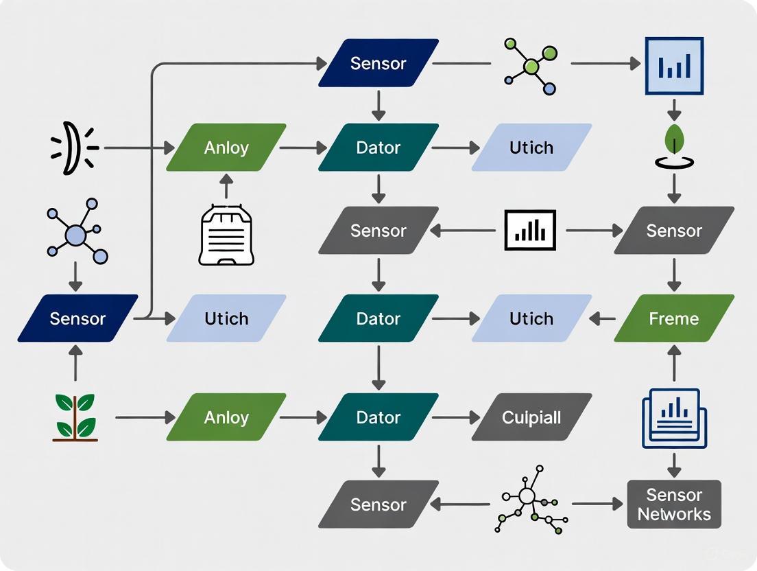
The following diagram illustrates the logical workflow and data signaling pathway from sensor data acquisition to intelligent control action in a research greenhouse network.
The Researcher's Toolkit: Essential Materials and Reagents
Table 2: Essential Research Reagents and Materials for Sensor Networks
| Item | Function/Application | Research-Grade Specifications |
|---|---|---|
| 4-in-1 Soil Sensor | Simultaneous in-situ measurement of soil moisture, temperature, pH, and EC [1]. | RS485 interface with MODBUS-RTU protocol; IP68 waterproof rating; ±0.5°C temp accuracy; ±3% FS EC accuracy [1]. |
| NDIR CO₂ Sensor | Precisely monitors carbon dioxide levels for photosynthesis studies [2] [3]. | Non-Dispersive Infrared technology with temperature/humidity compensation; accuracy of ±30 ppm [2]. |
| PAR Light Sensor | Measures Photosynthetically Active Radiation (400-700 nm) crucial for plant growth studies [3]. | Calibrated to measure photosynthetic photon flux density (PPFD) in µmol/m²/s; spectral response matched to plant absorption. |
| pH Buffer Solutions | For accurate calibration of pH sensors to ensure data validity [2]. | Certified standard solutions (e.g., pH 4.01, 7.00, 10.01) with known uncertainty values. |
| Conductivity Standard | For precise calibration of Electrical Conductivity (EC) sensors [2]. | Aqueous solution of known conductivity (e.g., 1413 µS/cm KCl solution at 25°C). |
| Data Acquisition Gateway | Aggregates data from multiple sensors for transmission to a central server [4]. | Supports multiple protocols (e.g., ZigBee, LoRaWAN, Wi-Fi); capable of edge computing and preprocessing [4]. |
The implementation of robust sensor networks is fundamental to modern greenhouse research, enabling precise environmental control for applications ranging from advanced agriculture to pharmaceutical development. Internet of Things (IoT) platforms integrate sensors, communication protocols, and data analytics to transform raw environmental data into actionable insights. Among the plethora of available wireless protocols, LoRaWAN, Zigbee, and Wi-Fi have emerged as prominent technologies for reliable data transmission in research settings. Each protocol offers a distinct set of trade-offs in range, power consumption, data rate, and network topology, making their selection critical to the success of a research deployment. This document provides detailed application notes and experimental protocols to guide researchers in implementing sensor networks that ensure data integrity and reliability within the context of greenhouse monitoring.
Protocol Technical Specifications and Comparative Analysis
Quantitative Protocol Comparison
Selecting an appropriate wireless communication protocol requires a clear understanding of technical specifications and their implications for a research environment. The following table summarizes the key quantitative and qualitative characteristics of LoRaWAN, Zigbee, and Wi-Fi.
Table 1: Comparative Analysis of Wireless Communication Protocols for Greenhouse Monitoring
| Feature | LoRaWAN | Zigbee | Wi-Fi |
|---|---|---|---|
| Frequency Band | 868 MHz (EU), 915 MHz (US) [5] | 2.4 GHz (Global), 868/915 MHz (Regional) [5] | 2.4 GHz, 5 GHz [6] |
| Range | Up to 15 km (rural), 2-5 km (urban) [6] [5] | 30 - 100 meters [5] | ~100 meters (indoors), ~300 meters (outdoors) [6] |
| Data Rate | 0.3 kbps to 50 kbps [6] [5] | 20 kbps to 250 kbps [5] | Up to several Gbps [6] |
| Power Consumption | Ultra-low (Battery life: years) [6] [5] | Low (Battery life: months to years) [5] | High (Requires frequent charging or constant power) [6] |
| Network Topology | Star [5] | Mesh, Tree, Star [5] | Star [6] |
| Typical Node Density | High (Thousands per gateway) [6] | High (Supports many devices in a mesh) [5] | Low to Medium (Congestion occurs with many devices) [6] |
| Key Strength | Long range, ultra-low power, deep signal penetration [5] | Reliable mesh networking, self-healing, low latency [7] [5] | High bandwidth, ubiquitous infrastructure [6] |
| Primary Limitation | Very low data rate, higher latency [6] [5] | Short range, complex configuration [5] | High power consumption, limited range, poor scalability [6] |
Application Context and Selection Guidelines
The choice of protocol is dictated by the specific requirements of the research application:
LoRaWAN is ideally suited for wide-area monitoring of large greenhouse complexes or remote research stations where power infrastructure is limited. Its long range and low power consumption make it perfect for sparse, periodic data collection from a large number of sensors, such as soil moisture, ambient temperature, and humidity [6] [8]. However, it is unsuitable for high-bandwidth applications like real-time video streaming or frequent control signals [6].
Zigbee excels in medium-range, high-density networks within a single greenhouse or a confined research area. Its mesh topology enhances reliability through self-healing capabilities; if one communication path fails, the network automatically reroutes data via an alternative path [5]. This is critical for monitoring and control systems where data integrity is non-negotiable, such as in pharmaceutical research environments [7]. Its moderate data rate supports more frequent sensor polling than LoRaWAN.
Wi-Fi should be employed primarily in small-scale, power-rich research setups where high-speed data transfer is paramount. It is a viable option for connecting high-fidelity sensors or cameras that generate large data volumes and are located in close proximity to existing network infrastructure [6]. Its high power consumption and poor scalability make it less desirable for large-scale, battery-operated sensor deployments [6].
Experimental Protocols for Sensor Network Implementation
Protocol 1: LoRaWAN Network Deployment for Spatial Environmental Monitoring
Objective: To establish a low-power, long-range sensor network for monitoring and predicting spatial environmental variations within a large research greenhouse [8].
Materials:
- LoRaWAN sensor nodes (e.g., for temperature, humidity, soil moisture, CO₂)
- LoRaWAN gateway with Ethernet/cellular backhaul
- LoRaWAN Network Server (e.g., The Things Network, ChirpStack)
- Cloud platform for data analytics and visualization
Methodology:
- Gateway Placement: Position the gateway at a central, elevated location within the greenhouse to maximize line-of-sight coverage. For very large or structurally complex greenhouses, multiple gateways may be required to ensure all sensor nodes have a reliable connection [8].
- Node Configuration:
- Configure all sensor nodes with the appropriate application and network keys for secure join-on activation [8].
- Implement Adaptive Data Rate (ADR). This algorithm automatically optimizes the data rate and transmission power for each node based on its link quality to the gateway, maximizing network capacity and battery life [8]. The typical power consumption for a LoRaWAN node can be as low as 7.66 µA in sleep mode [8].
- Set an appropriate data transmission interval (e.g., every 10-15 minutes) to balance data granularity with power consumption [8].
- Data Workflow: Sensor nodes collect and transmit data to the gateway via LoRa modulation. The gateway forwards this data to the LoRaWAN Network Server, which manages the network and forwards the decrypted payload to the designated cloud application for storage, analysis, and visualization [8].
- Performance Validation: Monitor the Signal-to-Noise Ratio (SNR) and Packet Delivery Rate (PDR). An SNR above 11.875 dB typically indicates a robust connection within 50-100 meters. A PDR of >99% should be targeted; rates as low as 40.9% have been reported at 700 meters in challenging conditions, highlighting the need for optimal gateway placement [8].
Protocol 2: Zigbee Mesh Network for High-Reliability Control Systems
Objective: To deploy a resilient, self-healing wireless sensor network for real-time environmental monitoring and control in a confined, high-value research compartment [7].
Materials:
- Zigbee modules (Coordinator, Router, and End Device types)
- Various sensors (temperature, humidity, etc.)
- Actuators (for irrigation valves, fan controls)
- Microcontroller unit (e.g., ARM7, JN5139)
Methodology:
- Network Topology Design: Implement a Wireless Mesh Network (WMN) topology. This structure involves Zigbee routers that relay data for other nodes, creating multiple redundant pathways and significantly enhancing network reliability and range compared to a simple star topology [7].
- Node Programming and Address Allocation:
- Initialize the network with a single Zigbee Coordinator [7].
- Deploy Zigbee Routers to form the mesh backbone. These devices cannot sleep and must be powered continuously [7].
- Configure Zigbee End Devices with sensors. These devices can enter sleep mode to conserve power and communicate only through their parent router or coordinator [7].
- Network addresses are automatically assigned based on a predefined formula involving network level (
Lm), maximum children (Cm), and maximum routers (Rm) [7].
- Implementing an Improved Routing Protocol (e.g., EMP-ZBR): To mitigate network congestion and balance energy use, employ an enhanced routing protocol that incorporates:
- Queue Cache Occupancy Ratio (
Qcr): The current queue length divided by the maximum queue length [7]. - Energy Consumption Ratio (
Ecr): The total energy consumed divided by the initial energy [7]. - Link Quality Indicator (LQI): A measure of the signal strength and quality [7]. Routes are selected based on a cost function that combines these metrics, rather than just the shortest hop count, leading to optimized network performance [7].
- Queue Cache Occupancy Ratio (
- Data Integrity Check: The system should employ CRC check codes in its data packets to verify data integrity upon receipt [9].
The Scientist's Toolkit: Essential Research Reagents and Materials
Successful implementation of a greenhouse sensor network requires careful selection of hardware and software components. The following table details key materials and their specific functions in a typical research deployment.
Table 2: Essential Research Materials for Greenhouse Sensor Network Implementation
| Item Category | Specific Examples | Research Function |
|---|---|---|
| Sensor Nodes | JN5139 microprocessor [9], ARM7 microprocessor [9] | The core processing unit of a sensor node, responsible for data acquisition from sensors, processing, and managing wireless communication protocols. |
| Communication Modules | LoRa RYLR998 Transceiver [10], Zigbee based on IEEE 802.15.4 [7] [5] | Hardware that provides the physical layer for wireless data transmission according to the specific protocol (LoRa, Zigbee, etc.). |
| Sensing Elements | Ambient temperature/humidity sensor, Soil moisture/EC sensor, Light sensor [11] | Convert physical environmental parameters (e.g., temperature, moisture, light) into analog or digital electrical signals for measurement. |
| Gateway/Base Station | LoRaWAN Gateway [11], Base station with GPRS module [9] | A critical hub that aggregates data from multiple sensor nodes and provides a backhaul connection to the internet or a central server via Ethernet, Cellular, or Wi-Fi. |
| Power Management | Solar panels, 4.2V Li-ion battery, Regulated power supply system [9] | Provides a stable and continuous power source, especially critical for remote, battery-operated nodes. Solar panels can extend operational life indefinitely. |
| Network Server & Cloud | LoRaWAN Network Server [8], Blynk IoT Platform [10] | The software infrastructure that manages the network, receives, decrypts, and processes sensor data, and makes it available for visualization and analysis via cloud applications. |
The strategic implementation of IoT sensor networks using LoRaWAN, Zigbee, or Wi-Fi is a cornerstone of advanced greenhouse research. The choice of protocol is not one of superiority but of application-specific suitability. LoRaWAN provides unparalleled range and power efficiency for extensive monitoring. Zigbee offers robust and reliable connectivity for dense, meshed control systems. Wi-Fi delivers high bandwidth where power and infrastructure are readily available. By adhering to the detailed experimental protocols and utilizing the appropriate toolkit outlined in this document, researchers can build reliable data transmission infrastructures. This ensures the integrity of the environmental data that is critical for rigorous scientific experimentation in greenhouse environments, ultimately supporting advancements in agriculture and pharmaceutical development.
The integration of advanced sensor networks, edge computing, and cloud platforms represents a paradigm shift in precision agriculture, enabling the sustainable intensification of food production within controlled environments [4]. Smart greenhouses, which leverage these technologies, have evolved from passive structures into intelligent ecosystems that autonomously maintain optimal growing conditions [12]. This architectural approach facilitates a transformative move from reactive manual management to predictive, data-driven cultivation, significantly enhancing resource efficiency, crop resilience, and yield [13]. For researchers and scientists, implementing a robust system architecture is foundational to conducting reliable and replicable greenhouse monitoring research. This document provides detailed application notes and experimental protocols for constructing such a system, framed within the context of academic and industrial research.
The end-to-end architecture for a smart greenhouse monitoring system is composed of three distinct but integrated layers: the Sensor Layer, the Edge Computing Layer, and the Cloud Platform Layer. The Sensor Layer is responsible for raw data acquisition from the environment and plants. The Edge Computing Layer performs time-sensitive data processing, filtering, and local control actuation. Finally, the Cloud Platform Layer handles long-term data storage, large-scale analytics, and user accessibility.
The logical data flow and key components of this architecture are visualized in the diagram below.
Sensor Node Layer: Design and Deployment
The sensor node layer forms the perceptual system of the architecture, responsible for capturing raw data on the greenhouse microclimate and plant physiology.
Core Sensor Technologies
A comprehensive multi-sensor monitoring network should include, but not be limited to, the following sensor types to capture a holistic picture of the greenhouse environment [14] [4]:
- Environmental Sensors: Measure the ambient air conditions. This includes temperature sensors (with high precision of ±0.1°C), relative humidity sensors, and carbon dioxide (CO₂) sensors for photosynthesis optimization.
- Light Sensors: Quantify the light available for plant growth. Photosynthetically Active Radiation (PAR) sensors measure light in the 400-700 nm range, crucial for calculating the Daily Light Integral (DLI).
- Soil/Root Zone Sensors: Monitor the conditions at the root level. These include soil moisture sensors (volumetric water content), soil temperature sensors, electrical conductivity (EC) sensors for nutrient levels, and pH sensors.
- Air Quality Sensors: Detect gases that can affect plant health or worker safety, such as ethylene (for fruit ripening) or ammonia [14].
- Water Management Sensors: Track irrigation system performance, including flow rate and pressure sensors to detect leaks or blockages [14].
Quantitative Sensor Performance Specifications
The following table summarizes the key performance parameters for common greenhouse sensors, based on current technological capabilities.
Table 1: Performance Specifications of Common Greenhouse Sensors
| Sensor Type | Measured Parameters | Typical Accuracy | Measurement Units | Key Characteristics |
|---|---|---|---|---|
| Temperature | Air Temperature | ±0.1°C to ±0.5°C [14] [4] | °C | Multi-zone monitoring, solar radiation shields [14] |
| Humidity | Relative Humidity | ±2% to ±3% [4] | %RH | Dew point and Vapor Pressure Deficit (VPD) calculation [14] |
| CO₂ | Carbon Dioxide Concentration | ±30 ppm to ±50 ppm | ppm | For photosynthesis optimization and safety [14] |
| Light/PAR | Photosynthetically Active Radiation | ±5% | μmol/m²/s | Spectral analysis for different growth stages [14] |
| Soil Moisture | Volumetric Water Content | ±3% | % | Measurement at multiple root zone depths [14] |
| Soil EC | Electrical Conductivity | ±5% | dS/m | Indicator of nutrient concentration and salinity [14] |
Communication Protocols for Sensor Networks
Sensor nodes transmit data to the edge gateway using various wireless protocols, each with distinct trade-offs in range, power consumption, and data rate [14] [4].
Table 2: Comparison of Wireless Communication Protocols
| Protocol | Typical Range | Power Consumption | Data Rate | Ideal Use Case in Greenhouse |
|---|---|---|---|---|
| LoRaWAN | Long-range (km) [14] | Very Low [14] | Low | Large-scale greenhouse facilities, sparse data updates |
| Zigbee | Short to Medium (10-100m) | Low [14] | Medium | Dense mesh networks of sensors in a confined area [4] |
| Wi-Fi | Medium (50m) | High [14] | High | Data-intensive applications (e.g., video, high-frequency sampling) [14] |
| Cellular (4G/5G) | Wide-area | High | High to Very High | Remote monitoring in areas without local network infrastructure [14] |
Experimental Protocol: Sensor Network Deployment and Calibration
Objective: To deploy a wireless sensor network (WSN) that provides spatially representative and accurate measurements of the greenhouse environment.
Materials:
- Wireless sensor nodes (e.g., based on LoRaWAN or Zigbee).
- Sensors for temperature, humidity, PAR, soil moisture, and CO₂.
- Edge gateway device.
- Calibration instruments (traceable to national standards).
- Mounting equipment (poles, stakes, radiation shields).
Methodology:
- Pre-Deployment Calibration: Before installation, calibrate all sensors against certified reference instruments in a controlled climate chamber. Document the baseline accuracy.
- Strategic Sensor Placement:
- Deploy sensors in a grid pattern to map microclimates, with higher density in areas known for variability [4].
- Position environmental sensors at crop canopy height and in representative locations, avoiding direct sunlight, water spray, or proximity to heating/cooling vents [14].
- Install soil sensors at multiple depths within the root zone of representative plants.
- Network Configuration:
- Configure sensor nodes to transmit data at a frequency appropriate for the parameter (e.g., every 5 minutes for temperature, every hour for soil moisture).
- Establish a communication link between the sensor nodes and the edge gateway, ensuring a stable signal strength across the entire greenhouse.
- Data Validation and Ongoing Maintenance:
- Perform a validation check by co-locating a research-grade sensor with a subset of the network nodes for a 24-hour period post-deployment.
- Implement a preventive maintenance schedule, including sensor cleaning and periodic calibration checks (e.g., every 6-12 months) to ensure long-term data integrity [14].
Edge Computing Layer: Intelligent Data Processing and Control
The edge computing layer brings computational power and data analysis directly into the greenhouse, enabling real-time responsiveness and reducing reliance on cloud connectivity [13].
Core Functions of the Edge Layer
- Real-time Data Filtering and Cleansing: Raw sensor data is often noisy. The edge layer applies filtering algorithms (e.g., Kalman filters, moving average filters) to smooth data and improve signal quality for reliable interpretation [4].
- Local Intelligence and Anomaly Detection: Deployed machine learning models can analyze incoming data streams to detect early signs of plant stress, equipment malfunction, or disease outbreaks based on environmental patterns [13].
- Immediate Actuation and Control: The edge device can execute pre-defined control logic, automatically adjusting ventilation, heating, cooling, or irrigation systems in response to real-time sensor readings without waiting for a round-trip to the cloud [13]. This is critical for maintaining stable conditions.
- Data Compression and Aggregation: Before transmission to the cloud, the edge device can aggregate high-frequency data into meaningful summary statistics, reducing bandwidth usage and cloud storage costs [13].
The workflow for data processing and decision-making at the edge is outlined below.
Experimental Protocol: Implementing an Edge-Based Climate Control Loop
Objective: To implement and validate a closed-loop control system at the edge that maintains greenhouse temperature within a target range.
Materials:
- Edge computing device (e.g., industrial microcomputer like Raspberry Pi, NVIDIA Jetson, or similar).
- Temperature sensor network.
- Actuators (e.g., vent motors, fan relays, heater valve controller) connected to the edge device's I/O ports.
- Programming environment (e.g., Python).
Methodology:
- System Modeling:
- Develop a simple linear model of the greenhouse temperature dynamics. This can be done empirically by analyzing historical data of temperature change in response to actuator states (e.g., vent opening, heater on/off).
- Control Algorithm Development:
- Implement a Proportional-Integral-Derivative (PID) or a simpler rule-based controller on the edge device. The input is the error (difference between target and actual temperature). The output is a command to the actuators.
- Example Rule:
IF temperature > 25°C THEN open vents by 20%; IF temperature > 28°C AND external temp < internal temp THEN activate exhaust fans.
- Deployment and Testing:
- Deploy the control algorithm on the edge device. Ensure safe hardware interfacing with actuators.
- Run a controlled experiment over 48-72 hours. Compare the temperature stability (e.g., standard deviation, time outside target range) against a period of manual or timer-based control.
- Data Logging and Analysis:
- The edge device should log the setpoint, actual temperature, and all actuator commands at a high frequency.
- Analyze the data to calculate performance metrics such as Integral of Absolute Error (IAE) and energy consumption, comparing the edge-based control to the baseline.
Cloud-Based Data Platform: Analytics and Accessibility
The cloud platform serves as the central repository for historical data, enabling large-scale analytics, long-term trend analysis, and remote access.
Core Platform Capabilities
- Data Storage and Management: Cloud databases store time-series data from all sensors, providing a unified source of truth [14].
- Advanced Analytics and AI: Cloud resources train complex machine learning and deep learning models for predictive tasks that are too computationally heavy for the edge, such as yield forecasting [12] or optimizing long-term climate strategies using Model Predictive Control (MPC) [15].
- Accessible Visualization and Dashboards: Web-based dashboards present data through charts, graphs, and status indicators. For research inclusivity, these dashboards must be designed with accessibility as a first-class requirement, using semantic HTML5 and WAI-ARIA compliance to ensure compatibility with screen readers [16].
- Interpretable AI and Natural Language Interfaces: To bridge the gap between complex AI decisions and growers, Natural Language Generation (NLG) interfaces can be integrated. These systems use Large Language Models (LLMs) to transform control decisions (e.g., from an MPC) into clear, actionable explanations [15].
Experimental Protocol: Cloud-Based Predictive Modeling for Yield Forecasting
Objective: To develop and validate a machine learning model on the cloud platform that predicts crop yield based on historical environmental and plant data.
Materials:
- Cloud computing instance (e.g., AWS EC2, Google Cloud VM).
- Database of historical sensor data (e.g., min/avg/max temperature, humidity, light integral, soil moisture).
- Corresponding historical yield records (e.g., harvest weight per plant or per square meter).
- Machine learning library (e.g., Scikit-learn, TensorFlow/PyTorch).
Methodology:
- Data Preparation:
- Extract and clean at least one full growing cycle of data from the cloud database.
- Perform feature engineering, creating daily or weekly aggregated features (e.g., average daytime temperature, total light integral, average VPD).
- Align the environmental features with the final yield data for each cultivation batch or greenhouse zone.
- Model Training:
- Split the data into training and testing sets (e.g., 80/20 split).
- Train several regression models (e.g., Random Forest, Gradient Boosting, Linear Regression) to predict yield from the engineered features.
- Use cross-validation on the training set to tune hyperparameters.
- Model Evaluation and Deployment:
- Evaluate the best-performing model on the held-out test set. Report key metrics such as Root Mean Squared Error (RMSE) and R² score.
- Deploy the validated model as an API on the cloud platform, allowing it to generate yield predictions based on current and historical data from active growing cycles.
- Interpretability and Reporting:
- Use feature importance analysis from the model to inform researchers about which environmental factors most strongly influence yield in their specific setup.
- Integrate the model's predictions into the research dashboard, potentially using the NLG interface to generate summary reports [15].
The Researcher's Toolkit: Essential Materials and Reagents
Table 3: Key Research Reagent Solutions and Essential Materials
| Item | Function/Application in Research |
|---|---|
| Calibrated Reference Sensors | Used for validating and periodically re-calibrating the deployed sensor network to ensure data accuracy and research integrity. |
| Programmable Edge Device | The core processing unit for implementing local control algorithms, data filtering, and machine learning models at the network edge. Examples include Raspberry Pi, NVIDIA Jetson, or BeagleBone. |
| Data Logging and Visualization Software | Platforms like Grafana, or custom dashboards (e.g., based on AccessiDashboard [16]) for real-time monitoring and analysis of sensor data streams. |
| Machine Learning Framework | Software libraries such as TensorFlow, PyTorch, or Scikit-learn for developing predictive models for climate optimization, yield forecasting, and anomaly detection. |
| Large Language Model (LLM) API | Used to build natural language interfaces that make complex AI control decisions interpretable to researchers and growers, enhancing trust and usability [15]. |
| Wireless Communication Modules | Hardware modules (e.g., LoRaWAN, Zigbee transceivers) that enable the construction of flexible, wire-free sensor networks for dense spatial monitoring. |
Understanding the Impact of Microclimates on Plant Physiology and Research Reproducibility
The precise control and monitoring of plant growth environments are fundamental to advancing research in plant biology, agriculture, and drug development from natural products. Microclimates—the climate conditions within a small, specific area that differ from the surrounding area—exert a profound influence on plant physiology and morphology. In controlled environments such as greenhouses, microclimatic heterogeneity can be a significant source of experimental error, undermining the reproducibility of research findings. This application note, framed within the broader objective of implementing robust sensor networks for greenhouse monitoring, details the critical effects of microclimates on plant physiology and provides standardized protocols to mitigate variability, thereby enhancing data quality and reliability.
Quantitative Evidence: Microclimatic Impact on Plant Physiology
Empirical studies consistently demonstrate that subtle variations in microclimatic factors can lead to significant phenotypic divergence. The following tables summarize key experimental data on these effects.
Table 1: Impact of Microclimatic Manipulations on Spring Phenology (Budburst) [17]
| Manipulation Type | Species Studied | Effect on Budburst Timing (vs. Control) | Key Interpretive Finding |
|---|---|---|---|
| Increased Bud Albedo (White-painted buds) | Fagus sylvatica (Beech), Fraxinus excelsior (Ash), Prunus avium (Cherry), Quercus robur (Oak) | Delay of up to +12 days | Temperature is sensed locally within each bud; altering radiant energy absorption directly impacts developmental rate. |
| Reduced Light (c. 70% shade) | Fagus sylvatica, Fraxinus excelsior, Prunus avium, Quercus robur | Delay of up to +12 days | Light condition (PAR) and its thermal consequences significantly modulate bud development. |
Table 2: Impact of Microclimatic and Resource Conditions on Autumn Phenology (Leaf Senescence) [17]
| Condition / Manipulation | Species Studied | Effect on Senescence Timing (vs. Control) | Key Interpretive Finding |
|---|---|---|---|
| Reduced Light (Shade) | Fagus sylvatica, Fraxinus excelsior, Prunus avium | Delay of up to +39 days | Suggests a sink-limitation model; reduced photosynthesis delays carbohydrate saturation. |
| High Nutrient Availability | Fagus sylvatica, Fraxinus excelsior, Prunus avium | Delay of up to +7 days | Enhanced sink strength (growth potential) extends leaf functional lifespan. |
| Reduced Precipitation (Drought) | Prunus avium (Cherry) | Delay of +7 days | Species-specific stress responses can alter phenological patterns. |
| Fagus sylvatica (Beech) | Advance of -7 days |
Table 3: Microclimatic Parameters within Tree Shelters and Physiological Effects on Quercus ilex [18]
| Microclimatic Parameter | Condition Inside Shelter (vs. Outside) | Physiological/Morphological Impact on Holm Oak Seedlings |
|---|---|---|
| Vapor Pressure Deficit (VPD) | Lower in dark shelters under mesic conditions; Higher in light shelters under xeric conditions. | Low VPD associated with high transpiration. High VPD under xeric conditions led to decreased mid-day xylem water potential. |
| CO₂ Concentration | Wide diurnal oscillations (respiration at night, rapid assimilation post-sunrise). | Indicates a tightly coupled plant-shelter system where plant gas exchange directly modifies the internal environment. |
| Light Transmittance | Reduced (Control > Light Shelter > Dark Shelter). | Increased plant height, leaf area, and shoot:root ratio under mesic conditions; morphological adaptations that may increase drought susceptibility. |
Experimental Protocols for Assessing Microclimate Effects
Protocol: Manipulating and Monitoring Bud-Level Microclimates
This protocol is adapted from controlled experiments to quantify the effect of localized microclimates on budburst phenology [17].
1. Objective: To determine the impact of bud albedo and light exposure on the timing of budburst in woody plant species. 2. Research Reagent Solutions & Materials:
| Item | Function/Brief Specification |
|---|---|
| White & Black Non-Toxic Paint | To manipulate bud albedo, altering the absorption of radiant energy. |
| Neutral-Density Shade Cloth | To reduce photosynthetically active radiation (PAR) by a defined percentage (e.g., 70%). |
| High-Resolution Digital Camera | For daily time-lapse imaging to visually track bud development stages. |
| Fine-Tip Thermocouples or IR Thermometer | To measure bud meristem temperature at high resolution. |
| Data Logger | To continuously record temperature data from sensors. |
| Phenology Score Sheet | Standardized chart for scoring bud stages (e.g., bud swell, bud break, leaf out). |
3. Methodology:
- Step 1: Experimental Setup. Select uniform, dormant saplings. Assign treatments to individual buds or plants in a fully randomized block design. Treatments include: (a) Control (unpainted buds, full light), (b) High Albedo (white-painted buds), (c) Low Albedo (black-painted buds), (d) Shade (plants/ buds under shade cloth).
- Step 2: Microclimate Monitoring. Install temperature sensors adjacent to target buds to record meristem-level temperature at hourly intervals. Simultaneously, record macro-climate data from a nearby station.
- Step 3: Phenological Observation. From the end of the chilling period, make daily visual observations or capture gigapixel time-lapse images [19]. Record the date when each bud reaches a predefined developmental stage (e.g., "budburst" as the first emergence of green leaf tip).
- Step 4: Data Analysis. Calculate the number of days to budburst for each treatment. Analyze data using ANOVA to determine significant effects of albedo and shade, correlating budburst timing with the recorded meristem temperature data.
Protocol: Integrated Sensor Network for Greenhouse Microclimate Monitoring
This protocol outlines the deployment of a wireless sensor network (WSN) for real-time, high-resolution environmental monitoring to identify and control for microclimatic variation [20].
1. Objective: To establish a WSN for capturing spatial and temporal heterogeneity in greenhouse microclimates, thereby improving experimental reproducibility. 2. Research Reagent Solutions & Materials:
| Item | Function/Brief Specification |
|---|---|
| Arduino Microcontroller (e.g., Mega) | Acts as the central processing unit for data from multiple sensors. |
| DHT11 Sensor | Measures air temperature and humidity. |
| Soil Moisture Sensors | Measures volumetric water content in the growth medium. |
| GSM/GPRS Module | Enables wireless transmission of collected data to a remote server. |
| PAR Sensor | Measures photosynthetically active radiation (400-700 nm). |
| Precision Irrigation System | Automated system for controlled water delivery; can be integrated via the network [21]. |
3. Methodology:
- Step 1: Network Design and Sensor Placement. Design a grid across the greenhouse growth area. Place sensor nodes at multiple heights (e.g., near the plant canopy, mid-canopy, and substrate level) and locations (center, edges, near vents) to capture 3D environmental gradients.
- Step 2: System Integration. Connect sensors to the Arduino microcontroller. Program the microcontroller to read sensor data at defined intervals (e.g., every 15 minutes). Integrate the GSM module for data transmission.
- Step 3: Data Acquisition and Visualization. Transmit data to a cloud server or central database. Use interactive software (e.g., a custom dashboard) to visualize real-time maps of temperature, humidity, and PAR across the greenhouse.
- Step 4: Actuation and Control. Use the sensor data as input for automated control systems. For example, trigger precision irrigation in response to substrate moisture thresholds or adjust shading based on real-time PAR readings [21]. This creates a closed-loop system to maintain homogenous conditions.
Implementation: A Workflow for Reproducible Greenhouse Research
The integration of microclimate awareness, sensor networks, and high-throughput phenotyping is essential for robust science. The following workflow diagram outlines this integrated approach.
Research Reproducibility Workflow
The Scientist's Toolkit: Essential Research Reagents and Materials
Table 4: Key Tools for Microclimate Monitoring and Plant Phenotyping [19] [20] [21]
| Category | Item | Critical Function |
|---|---|---|
| Sensor Network Components | Arduino Microcontroller (e.g., Mega) | Low-cost, programmable central processing unit for data acquisition and control. |
| DHT11/22 Sensor | Measures fundamental air parameters: Temperature and Humidity. | |
| Soil Moisture Sensor | Measures volumetric water content at root zone. | |
| Photosynthetically Active Radiation (PAR) Sensor | Quantifies light available for photosynthesis. | |
| GSM/GPRS Module | Enables remote, wireless transmission of sensor data. | |
| High-Throughput Phenotyping | Gigapixel Time-Lapse Camera System | Enables ecosystem-scale phenotyping with high spatial/temporal resolution [19]. |
| 3D Laser Scanner (e.g., PlantEye) | Automates non-destructive measurement of morphological parameters (e.g., leaf area, digital biomass) [21]. | |
| Multispectral Imaging Sensor | Captures physiological data (e.g., NDVI) beyond human vision by combining 3D and spectral data [21]. | |
| Experimental Materials | Neutral-Density Shade Cloth | Precisely controls light exposure levels for experimental treatments. |
| Tree Shelters | Creates defined microclimates for studying plant-shelter interactions (e.g., VPD, CO₂ oscillation) [18]. | |
| Precision Irrigation System | Automates and controls water delivery, integrating with sensor data for closed-loop feedback [21]. |
Microclimatic variation is an unavoidable reality in biological research that, if unaccounted for, systematically undermines data integrity and reproducibility. The implementation of a dense wireless sensor network is no longer a luxury but a necessity for characterizing the true environment in which plants grow. When combined with high-throughput, non-destructive phenotyping platforms, researchers can move beyond simply documenting final yields to understanding the dynamic physiological responses of plants to their immediate environment. By adopting the protocols and tools outlined in this document, researchers can significantly enhance the rigor, reliability, and reproducibility of their work, accelerating progress in plant science and drug development.
In the realm of controlled environment agriculture (CEA) research, the precise quantification of system performance is paramount. For research-grade greenhouse systems, two Key Performance Indicators (KPIs) stand out for assessing productivity and efficiency: Yield per m² and Energy per kg. These metrics provide researchers with critical insights into the interplay between agricultural output and resource consumption, enabling data-driven optimization of cultivation protocols. Yield per m² serves as the foremost indicator of production efficiency and success in optimizing greenhouse space for maximum output [22]. Energy per kg (or per pound) provides critical insight into operational cost structure and environmental impact, calculating the direct energy expense associated with producing one unit of sellable product [22]. Within the context of a broader thesis on implementing sensor networks for greenhouse monitoring, these KPIs transform raw sensor data into actionable intelligence for system optimization.
Quantitative KPI Benchmarks and Frameworks
Establishing well-defined KPIs requires standardized formulas and benchmark values to enable meaningful comparison and goal-setting. The following frameworks are essential for normalizing performance data across different research setups.
Table 1: Core Productivity and Efficiency KPI Definitions
| KPI | Formula | Unit | Research Application |
|---|---|---|---|
| Yield per m² [22] | Total Harvest Weight (kg) / Growing Area (m²) | kg/m² | Measures production efficiency and spatial optimization. |
| Energy per kg [22] | Total Energy Consumed (kWh) / Total Harvest Weight (kg) | kWh/kg or $/kg | Assesses energy cost efficiency and environmental impact. |
| Energy Intensity [23] | Total Energy Consumption / Unit of Activity | kWh/Unit | Reveals operational efficiency relative to output. |
| Carbon Intensity [23] | Total GHG Emissions (CO2e) / Unit of Activity | kg CO2e/Unit | Links energy use to carbon footprint for sustainability studies. |
Table 2: Industry Benchmark Ranges for Common Crops
| Crop Type | Yield per m² Benchmark (kg/m²/year) | Energy per kg Benchmark (kWh/kg) | Notes |
|---|---|---|---|
| Tomatoes [22] | 40 - 50+ | Varies with climate control | Top performers can exceed 50 kg/m². |
| Lettuce (Hydroponic) [22] | 39 - 49 (approx. 8-10 lbs/sq ft) | -- | High-density systems can achieve superior yields. |
| General Produce [22] | -- | 0.25 - 1.00 (approx. $0.15-$0.60/lb) | Highly dependent on local energy costs and climate. |
The European UNION’s LEVEL(S) framework provides a standardized methodology for evaluating sustainability performance, emphasizing the need for clearly defined metrics and thresholds to gauge target achievement effectively in building-related research, a principle that applies directly to greenhouse structures [24]. Furthermore, tracking carbon emissions as a KPI is increasingly crucial, with Scope 1 (direct emissions from owned sources like gas boilers) and Scope 2 (indirect emissions from purchased electricity) being the primary focus for initial reporting [25].
Experimental Protocols for KPI Data Acquisition
Reliable KPI calculation depends on rigorous, repeatable methodologies for data collection. The following protocols outline standardized procedures for acquiring the primary data streams required.
Protocol for Yield per m² Measurement
Objective: To accurately determine the biomass output per unit area of a greenhouse research system. Materials: Calibrated weighing scale, measuring tape or laser distance meter, data logging software. Methodology:
- Define Harvest Unit: Clearly specify the harvestable unit (e.g., whole plant, marketable fruit, fresh weight, dry weight).
- Demarcate Test Area: Precisely measure and mark the growing area (in m²) dedicated to the crop under study.
- Harvest and Log: At the end of the growth cycle, harvest the produce from the defined test area.
- Weigh and Record: Immediately weigh the total harvest using a calibrated scale and record the value.
- Calculate: Apply the formula:
Yield per m² = Total Harvest Weight (kg) / Growing Area (m²).
Protocol for Energy per kg Measurement
Objective: To quantify the total energy consumed per unit of harvested biomass. Materials: Sub-metering equipment on all major energy loads (HVAC, lighting, pumps), data acquisition system, calibrated weighing scale. Methodology:
- Install Sub-meters: Implement sub-metering at the most basic level to distinguish energy used in the growing area from other loads (e.g., office space) [25]. This provides a granular view of energy usage and carbon intensity.
- Define System Boundary: Specify whether the study includes only direct climate control energy or also ancillary loads (e.g., nutrient dosing, monitoring systems).
- Monitor Concurrently: Record total energy consumption (in kWh) from the sub-meters throughout the entire growth cycle of the crop being studied.
- Measure Yield: Follow Protocol 3.1 to obtain the total harvest weight (kg).
- Calculate: Apply the formula:
Energy per kg = Total Energy Consumed (kWh) / Total Harvest Weight (kg).
Sensor Network Architecture for KPI Monitoring
The accurate derivation of these KPIs relies on a robust sensor network that provides high-fidelity, real-time environmental and resource data.
System Design and Topology
A wireless sensor network (WSN) is fundamental for modern greenhouse research. A Wireless Mesh Network (WMN) topology is highly recommended for its resilience and scalability [7]. In this topology, router nodes can communicate directly with each other, preventing a single point of failure and enabling the network to cover large greenhouse areas effectively [7]. The network typically comprises:
- Sensor Nodes: Measure parameters like indoor/outdoor humidity and temperature, interior CO₂, and luminosity [26].
- Router Nodes: Relay data within the mesh network.
- Sink Node/Gateway: Aggregates data and connects the network to an edge server or cloud platform [26] [7].
The improved Zigbee routing protocol EMP-ZBR has been shown to optimize network performance by reducing end-to-end delay and increasing packet delivery rates, which is critical for reliable data acquisition [7].
Data Flow and AI-Enhanced Reliability
The integration of IoT and cloud computing enables sophisticated data handling and fault tolerance.
A key advancement is the use of AI for sensor fault detection and data imputation. As demonstrated in research, 1D Convolutional Neural Networks (CNNs) can be trained on long-term sensor data to predict values for faulty sensors based on correlations with other functional sensors [26]. This provides fault tolerance, ensuring the continuity and reliability of the data stream required for accurate KPI tracking, even when individual sensors fail [26].
The Scientist's Toolkit: Essential Research Reagent Solutions
The following table details key hardware, software, and methodological components essential for implementing a sensor network and calculating the core KPIs in a research context.
Table 3: Essential Research Reagents and Solutions for Greenhouse KPI Studies
| Item Name | Type | Function/Application in Research |
|---|---|---|
| Zigbee-based Sensor Node [7] | Hardware | Forms the basis of a low-power, wireless sensor network (WSN) for distributed environmental monitoring. |
| 1D CNN Fault Detection Model [26] | Software/Algorithm | Provides fault-tolerance by imputing accurate data for malfunctioning sensors, ensuring data integrity. |
| Sub-metering System [25] | Hardware | Enables granular tracking of energy consumption specifically for the growing environment, which is crucial for calculating "Energy per kg". |
| EMP-ZBR Routing Protocol [7] | Protocol/Algorithm | An improved Zigbee routing protocol that reduces network congestion and delay, enhancing WSN reliability and data delivery rates. |
| IoT Platform (e.g., Blynk) [27] | Software/Platform | Enables remote, real-time monitoring of sensor data and manual/automatic control of greenhouse components via a mobile application. |
| Natural Language Generation (NLG) Interface [15] | Software/Interface | Bridges the gap between complex AI control decisions (e.g., MPC) and researcher understanding by providing clear, actionable explanations. |
| LEVEL(S) Framework [24] | Methodological Framework | Provides a standardized EU methodology for setting thresholds and evaluating broader environmental sustainability, including energy and carbon. |
From Theory to Practice: A Step-by-Step Deployment and Integration Strategy
The implementation of a robust sensor network is a foundational pillar of modern greenhouse monitoring research. Moving beyond simple data collection, strategic sensor placement is critical for generating high-fidelity, spatially representative data on the microclimate at the canopy level, where plants interact with their immediate environment. Effective placement overcomes the limitations of traditional methods, which often rely on sparse, manual measurements that fail to capture the environmental heterogeneity within a greenhouse [4] [28]. This document provides detailed application notes and experimental protocols, framed within a broader thesis on implementing sensor networks for greenhouse research. It is designed to equip researchers and scientists with the methodologies needed to deploy sensors that yield accurate, actionable data for optimizing plant growth, health, and resource use in controlled environment agriculture.
Foundational Principles of Strategic Placement
Strategic sensor placement moves from arbitrary positioning to a data-driven methodology. The core principle is to deploy a limited number of sensors in locations that maximize the information gain relevant to specific research questions, whether concerning canopy-level climate gradients, water use efficiency, or disease prediction.
The design philosophy should balance several key factors:
- Spatial Representativeness: Sensors must capture the environmental variability across the entire greenhouse volume, not just a single point. This involves considering the three-dimensional nature of the canopy and the factors that drive microclimate formation [29].
- Data Redundancy and Resilience: A well-designed network should have a degree of redundancy to mitigate the impact of individual sensor failures, which can lead to data gaps and fragmented network coverage [4].
- Cost and Feasibility: While dense sensor carpets are ideal, they are often prohibitively expensive. The "hotspot" strategy demonstrates that greater predictive power can be achieved by strategically placing sensors in key locations rather than aiming for uniform, basin-wide coverage [30].
- Multi-Sensor Fusion: Integrating data from different sensor types (e.g., temperature, humidity, light, CO₂) provides a more holistic understanding of the environment. However, this introduces challenges in data synchronization, calibration, and interoperability that must be addressed in the experimental design [4] [31].
Sensor Placement Strategies and Protocols
This section outlines specific, actionable protocols for deploying sensors based on different research objectives.
Protocol 1: Multi-Zone Mapping for Canopy-Level Gradients
This protocol is designed to characterize the vertical and horizontal environmental gradients within the plant canopy.
- Objective: To quantitatively map the spatial variability of key microclimate parameters (temperature, humidity, light, CO₂) across the greenhouse canopy.
- Experimental Workflow: The following diagram illustrates the sequential workflow for this protocol.
- Detailed Methodology:
- Grid Definition: Divide the greenhouse into a three-dimensional grid. The horizontal resolution should be based on the scale of environmental variability, often starting with a zone every 50-100 square meters [4]. Vertically, place sensors at least at two critical heights: within the dense foliage of the canopy (e.g., 2/3 of plant height) and just above the canopy top.
- Sensor Deployment: Deploy identical, calibrated sensor suites at each grid vertex. Each node should, at a minimum, measure air temperature and relative humidity (e.g., DHT22, ±0.5°C, ±2%) [28] and photosynthetically active radiation (PAR). For more advanced studies, include CO₂ sensors.
- Data Collection: Collect data from all nodes simultaneously over a period that captures diurnal cycles (minimum 48-72 hours). The data should be timestamped and synchronized.
- Data Analysis: Use geostatistical methods (e.g., Kriging) to interpolate between sensor points and create contour maps (heat maps) of each environmental variable.
- Validation: Conduct mobile transect measurements with a portable sensor station to validate the interpolated maps from the fixed sensor network.
Protocol 2: Hotspot Monitoring for Predictive Modeling
This protocol adapts the strategic placement concept from snow hydrology to greenhouse environments, identifying and monitoring locations with the highest predictive value for specific outcomes [30].
- Objective: To identify "microclimate hotspots"— localized areas whose conditions are most predictive of broader greenhouse performance or plant stress—and deploy sensors for continuous, predictive monitoring.
- Experimental Workflow: The logic of identifying and utilizing these hotspots is shown below.
- Detailed Methodology:
- Baseline Data Collection: Begin with a high-resolution multi-zone mapping exercise (Protocol 1) to understand the baseline spatial variability.
- Correlation Analysis: Statistically correlate the sensor data from each location with relevant plant physiology data (e.g., leaf area index, stomatal conductance, fruit yield) or system-level outcomes (e.g., energy consumption, disease outbreak).
- Hotspot Identification: Identify the 3-5 sensor locations where environmental conditions showed the strongest statistical correlation with the outcomes of interest. These are the candidate "hotspots."
- Permanent Deployment: Install low-cost, permanent sensor nodes (e.g., based on ESP8266/NodeMCU) at these hotspot locations for continuous data streaming [32].
- Model Integration: Feed the real-time data from these hotspot sensors into a predictive model to forecast events like botrytis risk (from humidity) or water stress, enabling proactive management.
Technical Implementation and Data Integrity
Sensor Node Architecture and Network Configuration
A typical sensor node for a research-grade WSN includes several integrated components [28]:
- Microcontroller Unit (MCU): The computational core (e.g., Arduino Uno, NodeMCU ESP8266) that manages sensors, processes data, and handles communication [32] [28].
- Sensing Unit: A suite of sensors for environmental parameters (see Table 2).
- Wireless Communication Module: Often integrated into the MCU (e.g., Wi-Fi on ESP8266) or separate (e.g., LoRaWAN, ZigBee), this module transmits data to a gateway [29] [28].
- Power Supply: This can be a wired power source, batteries, or a solar-harvesting system for full energy autonomy, which is critical for remote or long-term studies [33].
Data Processing and Fault Detection
Raw sensor data is often noisy and requires processing to be useful. Researchers should implement embedded algorithms for initial data refinement.
Table 1: Common Data Filtering Techniques for Sensor Data Integrity
| Filtering Method | Principle | Best Use Case in Greenhouse Monitoring | Computational Load |
|---|---|---|---|
| Moving Average | Smooths data by averaging a sliding window of recent points. | Reducing high-frequency noise in temperature and humidity readings. | Low |
| Kalman Filter | Optimally estimates system state by combining predictions with noisy measurements. | Fusing data from multiple sensors and providing accurate estimates in dynamic conditions. | Medium to High |
| AI-Based Filtering | Uses machine learning models to identify and correct for anomalies and drift. | Complex fault detection (e.g., sensor drift, sudden failures) and predicting missing data. | High (requires training) |
| Hybrid Models | Combines two or more techniques (e.g., Kalman + AI). | Maximizing data integrity and system resilience for mission-critical research. | Very High |
For robust long-term experiments, an anomaly detection module is recommended. One effective approach is using the Isolation Forest algorithm, an unsupervised learning method that can be trained on synthetic data representing fault scenarios (e.g., irradiance drop, sensor drift, voltage imbalance) to identify anomalous readings in real-time data streams [33].
The Researcher's Toolkit
Table 2: Essential Research Reagent Solutions and Materials for Sensor Deployment
| Item / Technology | Function / Rationale | Research-Grade Considerations |
|---|---|---|
| DHT22 / AM2306 | Digital sensor for temperature and humidity measurement. | Higher accuracy and stability (±0.5°C, ±2-5% RH) compared to DHT11. Requires periodic calibration. [28] |
| BH1750FVI | Digital light intensity sensor for PAR measurement. | Spectral response should be matched to plant photosynthetic response. Critical for light-stress studies. |
| LoRaWAN Communication | Long-range, low-power wireless protocol. | Ideal for large greenhouses or areas with poor Wi-Fi; enables years of battery life. Reduces cabling infrastructure. [29] |
| Isolation Forest Algorithm | Unsupervised machine learning for anomaly detection. | Must be trained on labeled fault data. Effective for identifying sensor drift, icing, or complete failure. [33] |
| Portable Calibration Kit | Field kit for calibrating temperature, humidity, and gas sensors. | Essential for maintaining data integrity and scientific rigor over long-term experiments. |
| Multi-Sensor Fusion Framework | Software architecture to combine data from LiDAR, spectral, and environmental sensors. | Provides a comprehensive view of plant-environment interactions (e.g., structure + physiology + microclimate). [34] [31] |
Strategic sensor placement transforms a greenhouse from a passively controlled space into a dynamic, data-rich research environment. By moving beyond a "carpet" approach and adopting the targeted methodologies outlined in these protocols—Multi-Zone Mapping and Hotspot Monitoring—researchers can generate significantly more meaningful data for modeling and controlling the plant environment. The integration of robust WSN technology, advanced data filtering, and anomaly detection ensures the reliability of the collected data. Adhering to these guidelines will enable the scientific community to advance the field of precision agriculture, leading to more resilient, efficient, and productive controlled environment systems.
Application Notes: Core Sensor Technologies and Data Fusion Architecture
Essential Sensor Suite for Hyper-Localized Monitoring
The foundation of a precision greenhouse monitoring network is a suite of sensors that measure the key environmental variables influencing plant growth and health. Table 1 summarizes the essential sensors, their measured parameters, and technical specifications for research-grade applications [35].
Table 1: Essential Sensor Suite for Greenhouse Monitoring Networks
| Sensor Type | Measured Parameter(s) | Optimal Accuracy for Research | Key Considerations |
|---|---|---|---|
| Temperature & Humidity | Air Temperature, Relative Humidity | T: ±0.5 °C; H: ±2% [4] | Directly affects transpiration and nutrient uptake [35]. |
| CO₂ | Carbon Dioxide Concentration | ±30 ppm (NDIR sensors) [35] | NDIR sensors with temperature/humidity compensation are preferred [35]. |
| Light & Color | Photosynthetically Active Radiation (PAR), Light Spectrum | Spectral range: 400-700 nm (PAR) [35] | Crucial for monitoring light quality (red/blue spectrum) [35]. |
| Soil Moisture | Volumetric Water Content | Varies by technology (Capacitive, FDR, TDR) [35] | Capacitive sensors are less affected by soil salinity [35]. |
| Electrical Conductivity (EC) | Nutrient Concentration in Soil/Solution | Maintainable within ±0.2 mS/cm [35] | Measures total dissolved salts for nutrient management [35]. |
| Soil pH | Soil/Solution Acidity | Maintainable within ±0.2 pH units [35] | Solid-state sensors offer longer lifespan than glass electrodes [35]. |
| Leaf Wetness | Surface Moisture Duration | N/A | Critical for predicting fungal disease outbreaks (e.g., Botrytis) [35]. |
| Wind Speed | Airflow Velocity | N/A | Protects structure and optimizes ventilation [35]. |
Multi-Sensor Data Fusion Techniques
Sensor fusion combines data from disparate sources to create information with less uncertainty than that provided by a single sensor [36]. For greenhouse environments, this is implemented at three primary levels:
- Data-Level Fusion (Low-Level): This technique involves the direct combination of raw data from multiple homogeneous sensors (e.g., fusing readings from several temperature sensors to reduce noise and obtain a more accurate average temperature). While it can provide the most accurate result, it requires significant communication bandwidth and is sensitive to sensor misalignment [36].
- Feature-Level Fusion (Mid-Level): In this approach, features are first extracted from the raw data of each sensor. These features (e.g., a mean value, a rate of change, a Fourier transform component) are then fused. This method reduces data volume compared to data-level fusion. For instance, temperature, humidity, and leaf wetness features can be combined into a single "disease risk" index [36].
- Decision-Level Fusion (High-Level): Each sensor or sensor type first processes its own data to make a local decision (e.g., "irrigation needed," "ventilation required"). These individual decisions are then fused by a meta-level classifier to make a final, more robust decision. This approach allows for the combination of highly heterogeneous sensors and is more tolerant to individual sensor failure [36].
Figure 1: Data fusion hierarchy in a multi-sensor network, showing the progression from raw data to control decisions.
Experimental Protocols
Protocol: Deployment and Calibration of a Hyper-Localized Sensor Grid
Objective: To establish a calibrated wireless sensor network (WSN) that provides spatially resolved environmental data across the greenhouse for hyper-localized control.
Materials:
- Research Reagent Solutions & Essential Materials: The following table details the key components required for the experiment [35] [37] [38].
Table 2: Essential Research Materials for Sensor Network Deployment
| Item | Function/Description | Research-Grade Example |
|---|---|---|
| Sensor Nodes | Multifunctional units with microprocessor, memory, and wireless comms. | Custom nodes with programmable sampling intervals. |
| Base Station/Network Coordinator | Aggregates data from all nodes and provides gateway to the internet [37]. | Raspberry Pi or similar SBC running network management software. |
| Calibration Standards | Reference materials for verifying sensor accuracy. | Certified pH buffer solutions, calibrated reference hygrometer. |
| Wireless Communication Protocol | Ensures reliable, low-power data transmission [37]. | LoRaWAN or ZigBee modules for long-range, low-power needs. |
| Power Supply | Powers sensor nodes, especially in non-solar locations. | Li-ion batteries with solar charging capability. |
Methodology:
- Network Design and Sensor Placement:
- Divide the greenhouse area into a grid, with one sensor node per 100-200 m² for commercial operations [35]. For research on microclimates, a higher density may be required.
- Deploy sensor nodes at the plant canopy level, as this is where plants experience their immediate environment [35]. For soil sensors, install multiple probes at different depths (e.g., 5 cm, 15 cm, 30 cm) to monitor root zone moisture distribution [35].
- Strategically place nodes to avoid interference from HVAC vents, doors, and direct irrigation spray.
Pre-Deployment Calibration:
- Temperature/Humidity: Calibrate against a NIST-traceable reference sensor in an environmental chamber across the expected operational range (e.g., 10°C to 40°C, 20% to 90% RH).
- pH/EC Sensors: Calibrate pH sensors using standard buffer solutions (e.g., pH 4.01, 7.00, 10.01). Calibrate EC sensors using standard conductivity solutions [35].
- CO₂ Sensors: Allow NDIR CO₂ sensors to warm up as per manufacturer's instructions and calibrate in a environment with known CO₂ concentration if possible [35].
Data Synchronization and Logging:
- Implement a time-synchronization protocol (e.g., using Network Time Protocol - NTP) across all nodes to ensure data streams are temporally aligned.
- Configure the base station to log timestamped data from all nodes, storing it in a structured database.
In-Situ Validation:
- Periodically (e.g., bi-weekly), collect manual spot measurements using portable, calibrated instruments at the location of a subset of sensor nodes to validate network accuracy and identify drift.
Protocol: Implementing an AI-Driven Closed-Loop Control System
Objective: To integrate the sensor network with a machine learning-based control system that automatically adjusts greenhouse actuators (irrigation, vents, lights) to maintain hyper-localized setpoints.
Materials:
- Multi-sensor network (from Protocol 2.1)
- Central server with GPU capability for model training
- Programmable Logic Controller (PLC) or IoT-enabled actuators (solenoid valves, vent motors, LED lights, CO₂ injectors)
- Software libraries (e.g., Python with Scikit-learn, TensorFlow/PyTorch, Node-RED for automation logic)
Methodology:
- Data Preprocessing and Feature Engineering:
- Apply data filtering techniques such as Kalman filters or moving average filters to raw sensor data to reduce noise and handle missing data points [4].
- Engineer temporal features (e.g., rolling means, rates of change) and spatial features (e.g., differences between adjacent sensor nodes) to enrich the dataset for the machine learning model.
Model Selection and Training:
- Algorithm Choice: Select a machine learning algorithm suitable for the control task. Random Forest (RF) is effective for non-linear classification and regression tasks and is widely used in fusion-based monitoring [39]. For more complex temporal patterns, Long Short-Term Memory (LSTM) networks can be employed.
- Training: Train the model on historical data where both environmental conditions (sensor readings) and optimal actuator states (e.g., valve on/off, vent position) are known. The model learns to predict the optimal control action based on real-time sensor inputs.
System Integration and Control Logic:
- Deploy the trained model on the central server to make real-time inferences.
- Establish a control loop as depicted in Figure 2. The model's output is translated into commands for the PLC, which then activates the appropriate actuators.
Figure 2: AI-driven closed-loop control system for hyper-localized environmental management.
- Validation and Performance Metrics:
- Setpoint Deviation: Measure the average absolute deviation of environmental parameters from their target setpoints (e.g., ±0.5°C for temperature).
- Resource Efficiency: Quantify the reduction in water and energy usage compared to a traditional timer-based control system. Automated systems can reduce water consumption by 25-50% [35].
- Crop Yield and Quality: Monitor key crop metrics (e.g., biomass, fruit yield, Brix levels) to assess the agronomic impact of the precision control system.
LoRa (Long Range) is a modulation technique utilizing Chirp Spread Spectrum (CSS), designed for long-range, low-power wireless communication [40] [41]. While LoRaWAN is a network protocol that uses LoRa hardware in a star-of-stars topology involving gateways and network servers [41] [42], Peer-to-Peer (P2P) LoRa communication establishes a direct link between two end-node devices without intermediary gateways [40] [42]. This approach is particularly valuable for remote greenhouse monitoring in areas lacking cellular or Wi-Fi infrastructure, as it simplifies the system while retaining the benefits of long-distance connectivity and minimal energy consumption [40] [10].
Technology and Hardware Selection
LoRa P2P vs. LoRaWAN
For research applications requiring direct sensor-to-data logger communication in isolated environments, P2P LoRa offers a more suitable architecture compared to the more complex LoRaWAN.
Table: Comparison of LoRa P2P and LoRaWAN Architectures
| Feature | LoRa P2P Communication | LoRaWAN Network |
|---|---|---|
| Network Topology | Point-to-Point | Star-of-Stars |
| Infrastructure Requirements | Two end-node devices | End-nodes, Gateways, Network Server |
| Cost | Lower (no gateway cost) | Higher (requires gateway infrastructure) |
| Flexibility | High for direct device links | Governed by network server |
| Ideal Use Case | Simple, direct data links in remote areas | Large-scale, cloud-connected IoT deployments |
Essential Research Reagent Solutions (Hardware)
A functional P2P LoRa setup for a sensor network requires specific hardware components, each serving a distinct function in the data acquisition and transmission chain.
Table: Essential Hardware for a LoRa P2P Sensor Node
| Component Category | Example Parts | Research Function |
|---|---|---|
| Microcontroller | ESP32, NodeMCU ESP8266, Arduino Uno [40] [10] | Acts as the central brain; interfaces with sensors, processes data, and controls the LoRa module. |
| LoRa Transceiver Module | Reyax RYLR998, RYLR993, Grove Wio E5 [40] [10] [42] | Performs the long-range wireless modulation and demodulation; the core of the P2P link. |
| Environmental Sensors | DHT22 (Temp/Humidity), Analog Soil Moisture, CO₂ Sensor [10] [43] | Acquires quantitative physical and chemical data from the greenhouse environment. |
| Power Supply | 3.3V Regulated Source, Battery Holder [40] | Provides stable, often battery-backed, power for remote, long-term deployment. |
| Interface & Display | USB to Serial TTL Module (FT232RL), 0.96" OLED Display [10] [43] | Enables configuration, debugging, and local data visualization. |
Quantitative Performance and Configuration Parameters
LoRa P2P Link Budget and Performance
Understanding the operational limits of the technology is crucial for planning a successful deployment. The following data, synthesized from experimental setups, provides key performance benchmarks.
Table: LoRa P2P Operational Parameters and Performance Metrics
| Parameter | Typical Value / Range | Notes & Context |
|---|---|---|
| Frequency Bands | 868 MHz (EU), 915 MHz (US), 433 MHz [40] [10] | Must comply with regional regulations. |
| Transmission Range | Up to 6-7 km (Ideal, Line-of-Sight) [10] | Tested with RYLR998 modules; varies significantly with environment. |
| Path Loss Model (Vegetated River) | Log-normal distribution [44] | Empirical model for environments with water and dense vegetation. |
| Power Consumption | ~26 mA in Transmit Mode [42] | Enables long-term battery operation (years). |
| Data Reporting Interval | e.g., Every 2 minutes [40] | Configurable; lower frequency extends battery life. |
Core AT Command Set for Configuration
LoRa modules are typically configured via AT commands sent over a UART interface. The following sequence is critical for initializing a P2P link [40] [10].
AT: Checks module connectivity. Expected response:OK.AT+OPMODE=1: Sets the module to proprietary (P2P) mode. Expected response:OK.AT+ADDRESS=<Addr>: Sets the device's unique address on the network (e.g.,1for transmitter,2for receiver). Expected response:OK.AT+BAND=<Freq>: Sets the operating frequency band (e.g.,923000000for 923 MHz). Expected response:RESET.AT+NETWORKID=<ID>: Sets the network ID. Both communicating devices must share the same Network ID. Expected response:OK[10].
Experimental Protocol: Greenhouse Deployment Workflow
The following diagram and protocol outline a standardized method for deploying a P2P LoRa network for greenhouse monitoring, synthesizing best practices from documented projects.
Figure 1: Workflow for deploying a P2P LoRa network in a greenhouse environment.
Hardware Assembly and Interfacing
Objective: To physically construct the sensor (transmitter) and data logger (receiver) nodes.
Transmitter Node (Sensor Unit):
- Connect the microcontroller (e.g., ESP32) to the LoRa module (e.g., RYLR993) as follows [40]:
- LoRa
3.3V→ ESP323.3V - LoRa
GND→ ESP32GND - LoRa
RX→ ESP32 PinD5 - LoRa
TX→ ESP32 PinD4
- LoRa
- Interface all relevant sensors (DHT22, soil moisture, etc.) to the microcontroller's appropriate analog or digital pins [10] [43].
- Connect a suitable antenna to the LoRa module.
- Connect the microcontroller (e.g., ESP32) to the LoRa module (e.g., RYLR993) as follows [40]:
Receiver Node (Gateway Unit):
- Assemble a second unit with a microcontroller and LoRa module using the same electrical connections.
- This unit should be connected to a device capable of forwarding data to the internet (e.g., via Wi-Fi) or storing it locally [10].
Firmware Development and Configuration
Objective: To program the operational logic for both the transmitter and receiver nodes.
Transmitter Firmware Protocol:
- Initialize the hardware serial port for the LoRa module.
- Use the
sendATCommandfunction to send the sequence of AT commands detailed in Section 3.2 to configure the module [40]. - In the main loop, periodically read data from all connected sensors.
- Package the sensor readings into a string or structured payload.
- Use the
AT+SEND=<Addr>,<Length>,<Message>command to transmit the data to the receiver's address [40] [10]. Example:AT+SEND=2,30,25.5,60,1024(sends temperature, humidity, and pressure to device at address 2).
Receiver Firmware Protocol:
- Similarly, initialize and configure the LoRa module with its own address and the same network ID and band as the transmitter.
- Continuously listen for incoming messages. The module will output a
+RCVmessage upon reception [10]. - Parse the received string to extract the sensor data.
- Forward the parsed data to an IoT cloud platform (like Blynk or MQTT) via Wi-Fi, or log it to an SD card [10].
Range Validation and Path Loss Modeling
Objective: To empirically verify the communication link's reliability across the intended deployment area.
Field Testing:
- Place the transmitter at a fixed location within the proposed greenhouse site.
- Gradually move the receiver away from the transmitter, noting the GPS coordinates or precise distance at each test point.
- Record the Received Signal Strength (RSSI) or, for greater accuracy, the RF power of the chirp signal itself for each distance [44]. Document the packet loss rate.
Data Analysis:
- Plot the received power (or RSSI) against distance on a log-scale.
- Fit a log-normal path loss model to the data, which is characteristic for such environments [44]. The model can be expressed as:
- ( PL(d) = PL(d0) + 10 \cdot n \cdot \log{10}(\frac{d}{d0}) + X\sigma )
- Where ( PL(d) ) is the path loss at distance ( d ), ( n ) is the path loss exponent, ( d0 ) is a reference distance, and ( X\sigma ) is a zero-mean Gaussian random variable representing shadowing [44].
- This model allows researchers to predict the maximum reliable range for their specific site conditions and plan node placement accordingly.
Network Architecture and Data Flow
The overall system architecture for a remote greenhouse monitoring setup involves both the P2P LoRa link and a subsequent internet connection for global data access.
Figure 2: End-to-end data flow from remote sensors to the end researcher.
The implementation of a sensor-actuator network is a critical advancement in modern greenhouse research, enabling a closed-loop control system that dynamically optimizes the growing environment. This integration is foundational for studies requiring precise environmental control for plant phenotyping, metabolic compound production, or stress response analysis. By linking real-time sensor data to automated physical adjustments, researchers can maintain specific set-points or complex environmental regimes with minimal human intervention, thereby enhancing experimental reproducibility and reliability [45]. The core of this system relies on a seamless flow of information from sensors that perceive the environment to controllers that process this data and, finally, to actuators that execute physical changes in irrigation, lighting, and HVAC systems [46].
This document provides detailed application notes and experimental protocols for establishing such an integrated control system within the context of a research greenhouse. It frames the technical integration within the broader paradigm of using reinforcement learning (RL) to not just automate, but continuously optimize greenhouse operations for energy efficiency and crop-specific outcomes [45].
Application Notes
System Architecture and Workflow
A fully integrated greenhouse automation system functions as a hierarchical cyber-physical system. The logical flow of data and control commands can be visualized as a continuous loop of perception, decision, and action.
The diagram below illustrates the core signaling and control workflow that forms the basis of an automated greenhouse system.
Diagram 1: Automated Greenhouse Control Loop. This diagram illustrates the closed-loop feedback system where sensor data drives actuator responses via a central control logic, creating a self-regulating environment.
Quantitative Actuator Selection Guide
Selecting the appropriate actuator is critical for translating control signals into effective physical movements. The required force, stroke length, and precision vary significantly across applications. The following table summarizes key performance metrics for common actuators used in research greenhouse systems, aiding in the selection process based on quantitative needs.
Table 1: Performance Specifications of Common Greenhouse Actuators
| Application | Actuator Model/Type | Key Performance Metrics | Control Interface | Primary Research Use Case |
|---|---|---|---|---|
| Ventilation & Louver Control | Actuonix P16 or T16 Track Actuator [47] | Stroke: Up to 200mmContinuous Force: 25-45 NSpeed: 5.5-11.5 mm/s | 12V DC, LAC Board, Arduino/Raspberry Pi | Modulating roof vents or side vents for temperature and humidity regulation. |
| Shade Clutch & Blackout Control | Actuonix L12 or P16 Actuator [47] | Stroke: 50-200mmForce: 15-45 NSpeed: 3.8-14 mm/s | 12V DC, LAC Board, Arduino/Raspberry Pi | Precisely adjusting light intensity for photoperiod or stress studies. |
| Valve Control (Irrigation, Dosing) | Actuonix PQ12 Actuator [47] | Stroke: 20mmForce: 12-22 NSpeed: 3.6-6.5 mm/s | 12V DC, LAC Board, Arduino/Raspberry Pi | Precise control of irrigation valves or nutrient/pH dosing valves. |
| Light Height Adjustment | Actuonix L12 or P16 Actuator [47] | Stroke: 50-200mmForce: 15-45 NSpeed: 3.8-14 mm/s | 12V DC, LAC Board, Arduino/Raspberry Pi | Maintaining optimal photon flux density by adjusting LED light distance from canopy. |
| Lift Gates & Larger Valves | WT-100 Light Lift Gate Actuator [48] | Torque: 29-72.8 ft.lbs. (breakaway)Stem Speed: Flexible (1:1 ratio)Power: 12 VDC, 2.5 Amp-Hr/day | Fused torque limits, HOA (Hand/Off/Auto) toggle, SCADA-ready | Automating larger irrigation turnouts or pump control stations. |
Sensor-Actuator-Control Logical Relationships
The integration of sensors, controllers, and actuators forms a network of logical relationships where specific environmental parameters trigger targeted actions. This matrix defines the core logic that governs the automated system.
Table 2: Sensor-Actuator Control Logic Matrix
| Sensor Type | Measured Parameter | Target Actuator | Control Action | Research Objective |
|---|---|---|---|---|
| Temperature Probe [49] | Air Temperature (°C) | Vent Actuator (e.g., P16) [47] | Open/Modulate vents to maintain set-point. | Study plant thermal stress responses. |
| Pyranometer | Light Intensity (PPFD) | Shade Clutch Actuator (e.g., L12) [47] | Deploy/retract shade cloth to modulate light. | Investigate photosynthetic efficiency. |
| Soil Moisture Sensor | Volumetric Water Content (%) | Irrigation Valve Actuator (e.g., PQ12) [47] | Open/close valve to maintain soil moisture. | Determine optimal irrigation regimes. |
| Humidity Sensor [49] | Relative Humidity (%) | HVAC Damper Actuator / Dehumidifier | Modulate air exchange or dehumidification. | Control pathogen pressure and transpiration rates. |
| CO2 Sensor | CO2 Concentration (ppm) | CO2 Dosage Valve Actuator | Inject CO2 to enrich atmosphere. | Maximize photosynthetic carbon fixation. |
| pH/EC Sensor | Nutrient Solution pH/EC | Dosing Pump Actuator (e.g., PQ12) [47] | Add acid/base or nutrients to correct levels. | Maintain precise hydroponic nutrient conditions. |
Experimental Protocols
Protocol 1: Calibration of an Integrated Ventilation Control System
Objective: To establish and validate a closed-loop control system that uses temperature sensors to actuate roof vents, maintaining a precise air temperature set-point.
Materials:
- Temperature/Humidity Sensor (e.g., TE Connectivity HTU series) [49]
- Data Acquisition (DAQ) Module (e.g., Arduino/Raspberry Pi with ADC)
- Programmable Logic Controller (PLC) or Microcontroller
- Linear Actuator (e.g., Actuonix P16) [47] with mounting hardware
- Power Supply (12V DC)
- Actuator Control Board (e.g., LAC Board) [47]
- Personal Computer with control software (e.g., Python, MATLAB/Simulink)
Methodology:
- Hardware Setup:
- Mount the temperature sensor at canopy height in a representative location, shielded from direct radiation.
- Install the linear actuator onto the greenhouse roof vent mechanism, ensuring smooth operation through the full range of motion.
- Connect the actuator to the LAC control board, and connect the board to a digital output of the PLC/microcontroller.
- Connect the temperature sensor to an analog input of the DAQ module.
- Software Configuration:
- Develop a Proportional-Integral-Derivative (PID) control algorithm within the control software. Define the temperature set-point (T_set).
- Program the control loop: Read sensor voltage, convert to temperature, compute error (E = Tset - Tmeasured), and execute the PID function to determine the actuator command signal (0-100%).
- Map the output command to a pulse-width modulation (PWM) signal for the LAC board to control actuator position proportionally.
- Calibration and Tuning:
- Manually test the full range of the actuator to determine the 0% (fully closed) and 100% (fully open) positions.
- Run the system with a conservative PID gain (Kp). Introduce a step-change in set-point and observe the system's response.
- Iteratively tune the PID gains (Kp, Ki, Kd) to achieve a fast response without overshoot or oscillation (critically damped behavior).
- Validation Experiment:
- Program a diurnal temperature regime (e.g., 25°C day / 18°C night) for 24-48 hours.
- Log the set-point, measured temperature, and actuator position at 1-minute intervals.
- Calculate performance metrics: Mean Absolute Error (MAE), Root Mean Square Error (RMSE), and integral of absolute error (IAE) between set-point and measured temperature.
Protocol 2: Implementation of a Reinforcement Learning Agent for Multi-Variable Optimization
Objective: To implement an RL-based controller that co-optimizes temperature and humidity set-points by learning control policies for vent and HVAC actuators, balancing crop growth goals with energy consumption.
Materials:
- All materials from Protocol 1.
- Additional actuators: HVAC damper actuators, misting system valves.
- Humidity sensor [49], energy meter (for HVAC system).
- Computer capable of running RL simulations (e.g., with Python, PyTorch, OpenAI Gym).
Methodology:
- Problem Formulation:
- State (s): Define the state vector as [Tinside, RHinside, Toutside, RHoutside, SolarRadiation, CO2, TimeofDay].
- Action (a): Define the action vector as [VentPosition, HVACPowerLevel].
- Reward (R): Design the reward function. A sample function is:
R = -[(T_target - T_inside)² + w₁*(RH_target - RH_inside)² + w₂*Energy_Consumed]wherew₁andw₂are weighting coefficients that balance the importance of climate accuracy versus energy use [45].
- Agent Training:
- Select an RL algorithm (e.g., Deep Q-Network - DQN, or Proximal Policy Optimization - PPO).
- Begin training the agent using a digital model (simulation) of the greenhouse to learn preliminary policies without risking real crops.
- Once the agent performs well in simulation, deploy it in the real greenhouse system, initially in a "shadow mode" where its actions are logged but not executed.
- Finally, run the agent in live control mode for short periods, closely monitored, to allow for fine-tuning with real-world data [45].
- Performance Evaluation:
- Compare the RL controller's performance against a traditional PID controller over a 7-day period.
- Key Metrics:
- Climate Stability: MAE of temperature and humidity.
- Energy Efficiency: Total kWh consumed by the HVAC and actuator system.
- Crop Performance: Plant growth rate or photosynthetic rate (if measured).
The following diagram outlines the iterative learning process of the RL agent within the greenhouse environment.
Diagram 2: Reinforcement Learning Control Workflow. This diagram shows the interaction cycle where an RL agent learns optimal control policies by taking actions and receiving rewards based on the resulting state of the greenhouse environment.
The Scientist's Toolkit: Essential Research Reagents and Materials
Table 3: Key Components for a Sensor-Actuator Research Platform
| Item Category | Specific Product/Model Example | Research Function |
|---|---|---|
| Data Acquisition | Arduino Mega 2560 / Raspberry Pi 4 | Serves as a low-cost, programmable hardware platform for reading sensors and outputting control signals in prototype systems. |
| Programmable Logic Controller (PLC) | Siemens S7-1200 / Allen-Bradley Micro800 | Provides an industrial-grade, reliable control core for full-scale greenhouse automation, handling multiple I/O points and communication protocols. |
| Linear Actuator | Actuonix PQ12 [47] | Provides precise, small-scale linear motion for tasks requiring high accuracy and low force, such as valve control for nutrient dosing. |
| Linear Actuator | Actuonix P16 [47] | A versatile actuator with greater force and stroke, suitable for medium-duty applications like operating vents, louvers, or adjusting grow lights. |
| Gate Actuator | WT-100 Light Lift [48] | Automates larger gates and valves in irrigation or water management systems with high torque requirements; SCADA-ready for system integration. |
| Actuator Controller | Actuonix LAC Board [47] | Simplifies the integration of actuators with microcontrollers by providing a built-in driver for precise position control via simple serial commands. |
| Temperature & Humidity Sensor | TE Connectivity HTU21D-F [49] | Accurately monitors the ambient growing climate, providing critical feedback for environmental control algorithms. |
| Differential Pressure Sensor | TE Connectivity MS5837-02BA [49] | Monitors air flow pressure in ducts and can be used for filter monitoring, ensuring HVAC system integrity. |
| Communication Protocol | MQTT (Message Queuing Telemetry Transport) | A lightweight IoT publish-subscribe network protocol that transports messages between devices and a central data broker with low bandwidth. |
Application Note: System Architecture for Greenhouse Data Management
Core Concept and Rationale
The integration of sensor networks with cloud platforms creates a powerful digital twin of the greenhouse environment, enabling precision agriculture at an unprecedented scale [14]. This architecture transforms raw sensor data into actionable insights through a seamless pipeline of collection, transmission, storage, and analysis. For researchers, this system provides both real-time monitoring capabilities and deep historical analysis tools, supporting complex research into plant physiology, optimization of growing protocols, and longitudinal studies of environmental interventions.
Quantitative Sensor Specifications for Research-Grade Monitoring
The foundation of any effective monitoring system is its sensor network. The following table summarizes the critical parameters, recommended sensor technologies, and research applications for comprehensive greenhouse monitoring.
Table 1: Essential Sensors for Greenhouse Research Monitoring
| Parameter | Recommended Sensor Technology | Accuracy & Range | Primary Research Applications |
|---|---|---|---|
| Temperature | PT-100 Stainless Steel Probe [50] | ±0.1°C [14] | Study of plant metabolic rates, respiration, and stress response. |
| Humidity | Digital Embedded Probe [50] | ±2% RH (5-95% RH) [50] | Transpiration studies, disease modeling (e.g., Botrytis). |
| CO₂ | Non-Dispersive Infrared (NDIR) [50] | ±30 ppm [50] | Photosynthesis efficiency, CO₂ enrichment trial analysis. |
| Light (PAR) | Photosynthetically Active Radiation Sensor [14] | Measured in μmol/m²/s [14] | Daily Light Integral (DLI) calculation, growth model calibration. |
| Soil Moisture | Capacitive or FDR Sensors [50] | N/A | Irrigation optimization, water-use efficiency studies. |
| Leaf Wetness | Surface Moisture Sensors [14] | N/A | Pathogen infection risk assessment and disease prevention. |
| Soil/Water pH | Solid-State Digital Sensors [50] | Maintainable within ±0.2 units [50] | Nutrient availability studies, root zone health monitoring. |
| Electrical Conductivity (EC) | Conductivity Probes [50] | Maintainable within ±0.2 mS/cm [50] | Nutrient solution management, salinity stress research. |
Protocol: End-to-End System Implementation
Phase 1: Sensor Network Deployment and Calibration
Objective: To establish a robust and accurate physical sensor layer across the greenhouse research environment.
Materials:
- Sensors as specified in Table 1.
- Wireless sensor nodes or data loggers.
- Calibration standards for each sensor type.
- Mounting equipment.
Procedure:
- Strategic Sensor Placement:
- Install sensors at the plant canopy level, as this is the microclimate directly experienced by the plants [50].
- For larger or multi-zone greenhouses, deploy multiple sensors to map environmental gradients (e.g., one sensor per 1,000-2,000 square feet) [14].
- Avoid placing sensors near direct HVAC vents, irrigation spray, or structural supports to ensure representative readings [14].
- For soil parameters, deploy sensors at multiple depths (e.g., 5cm, 15cm, 30cm) to monitor moisture distribution through the root zone [50].
Pre-Deployment Calibration:
- pH and EC Sensors: Calibrate using standardized buffer solutions (e.g., pH 4.0, 7.0, 10.0) and conductivity standards prior to installation [50].
- CO₂ Sensors: Perform calibration as per manufacturer instructions, often involving a zero-point calibration [50].
- All Sensors: Document all calibration dates and standard values for traceability.
Network Connectivity Verification:
- Power on all sensor nodes and verify their connection to the central gateway.
- Confirm a strong and stable signal strength for wireless sensors across the entire facility to prevent data gaps [50].
- Establish a unique naming convention for each sensor (e.g.,
GH1_North_Zone_Temp) within the data management platform.
Phase 2: Data Transmission and Cloud Ingestion
Objective: To reliably transmit sensor data from the greenhouse to a cloud-based data platform for processing and storage.
Materials:
- Gateway device.
- Cloud platform account (e.g., Google Cloud, AWS).
- Configured data pipelines.
Procedure:
- Select Communication Protocol: Choose a wireless protocol based on range, power consumption, and data rate requirements. Common research choices include:
- Configure Data Ingestion Pipeline:
- Utilize cloud services to create a streaming data pipeline (e.g., Google Cloud's Pub/Sub or AWS IoT Core).
- Ingest data from the gateway into a cloud storage optimized for analytics, such as Google BigQuery or a time-series database [51].
- Implement a data validation step in the pipeline to flag and quarantine outlier or physically impossible readings.
Phase 3: Cloud-Based Data Management and Analysis
Objective: To store, process, and analyze the ingested sensor data to generate insights.
Materials:
- Cloud data platform (e.g., Google BigQuery, Bigtable).
- Analytics and visualization tools.
Procedure:
- Implement a Hybrid Storage Architecture:
- Use a real-time analytics database like Google Bigtable for low-latency, user-facing applications and fast retrieval of recent data [51].
- Use a cloud data warehouse like Google BigQuery for complex historical analysis and aggregations over the entire dataset [51].
- Leverage the seamless integration between these systems to run complex SQL queries that combine real-time and historical data [51].
- Develop Analytical Models:
- Real-Time Analytics: Create dashboards that update in seconds, displaying key performance indicators (KPIs) like current environmental conditions and system status [52]. This enables immediate response to threshold violations.
- Historical Analysis: Perform batch analysis in the data warehouse to identify long-term trends, correlations between environmental parameters and crop yield, and the efficacy of different growing protocols [53].
- Predictive Analytics: Apply machine learning models to the historical dataset to forecast outcomes, such as predicting disease risk based on trends in humidity and leaf wetness [53].
Phase 4: Dashboard Creation for Real-Time Monitoring and Historical Review
Objective: To visualize data for both operational awareness and in-depth research analysis.
Materials:
- Data visualization tool (e.g., Looker Studio, Kibana [54]).
Procedure:
- Design Real-Time Dashboards:
- Use a tool like Kibana to create visualizations that update every few seconds [54].
- Incorporate a variety of widgets: gauge charts for immediate status (e.g., current temperature), line charts to show trends over the last hour, and tables that can be sorted and filtered [55].
- Set a global time filter, for example, to show the "Last 15 minutes" or "Today" [54].
- Configure color-coded thresholds to provide instant visual cues for out-of-range conditions [55].
- Develop Historical Analysis Dashboards:
- Connect your visualization tool directly to the cloud data warehouse (BigQuery).
- Create line and stacked-area charts to visualize environmental trends over weeks or months [55].
- Use heatmap charts to visualize distribution-valued metrics, such as the variation in temperature across different zones in a 24-hour period [55].
- Pair charts with detailed tables to allow researchers to drill down from a observed anomaly to the underlying raw data [55].
The Scientist's Toolkit: Essential Research Reagents and Solutions
Table 2: Key Components for a Greenhouse Data Management System
| Item / Solution | Function in Research Context |
|---|---|
| NDIR CO₂ Sensor | Provides accurate, stable measurements of carbon dioxide levels essential for photosynthesis studies and enrichment trials. Superior to electrochemical sensors for research-grade accuracy [50]. |
| PAR Light Sensor | Precisely measures Photosynthetically Active Radiation (μmol/m²/s) for calculating Daily Light Integral (DLI), a critical factor in growth model development [14]. |
| Leaf Wetness Sensor | Detects surface moisture on plant canopies, enabling quantitative research into microclimate conditions that promote pathogen growth and disease development [14]. |
| Multi-Depth Soil Moisture Probes | Monitors water content at various root zone depths, providing data for studies on plant water uptake patterns and irrigation protocol efficiency [50]. |
| LoRaWAN Communication Module | Enables long-range, low-power wireless sensor connectivity across large research greenhouses or field trials, minimizing infrastructure costs [14]. |
| Cloud Data Warehouse (BigQuery) | Serves as the central repository for all historical sensor data, enabling complex SQL queries, multivariate analysis, and long-term trend identification [51]. |
| Real-Time Analytics DB (Bigtable) | Powers low-latency applications and dashboards, allowing researchers to observe and react to experimental conditions as they happen [51]. |
| Containerized Analytics Platform | Provides a flexible and portable environment (e.g., on Kubernetes) for deploying custom data processing, machine learning models, and analysis pipelines [53]. |
Ensuring Data Integrity: Advanced Calibration, Filtering, and Anomaly Management
Implementing a robust sensor network is fundamental to modern greenhouse research, enabling the precise microclimate control needed for experimental repeatability and high-quality yields [4]. The foundation of any data-driven research system is data integrity; reliable data is crucial for the analysis, monitoring, and forecasting of system behavior, whereas poor-quality data can lead to erroneous conclusions and flawed scientific models [56]. Greenhouse environments present a unique set of challenges for maintaining this integrity. The internal conditions can be harsh for electrical sensors, exposing them to water, high solar radiation that can heat the devices, and connectivity issues that lead to data loss [57]. Furthermore, the dense deployment of nodes often needed for comprehensive monitoring can lead to sensors sensing similar data, creating data redundancy at the sink node [56].
This document outlines the common data quality challenges—sensor noise, redundancy, inconsistencies, and missing data—within the context of greenhouse monitoring for research and drug development. It provides application notes and detailed experimental protocols to help researchers identify, quantify, and mitigate these issues, thereby ensuring the collection of high-fidelity data for critical analyses.
Selecting appropriate sensors is the first step in mitigating data quality issues. The table below summarizes common sensor types used in greenhouses and their typical performance characteristics, which directly influence data quality.
Table 1: Common Greenhouse Monitoring Sensors and Performance Characteristics
| Sensor Type | Measured Parameter | Common Technology | Typical Accuracy/Notes | Primary Data Challenge |
|---|---|---|---|---|
| Temperature | Air/Soil Temperature | Thermistor | ±0.1°C to ±0.5°C; quick response [3] | Noise, Calibration Drift [4] |
| RTD | ±0.1°C or better; high stability [3] | |||
| Thermocouple | ±1°C to ±2°C; durable for harsh conditions [3] | |||
| Humidity | Relative Humidity | Capacitive | Fast response, low maintenance, high accuracy [3] | Inconsistencies across locations [4] |
| Resistive | Cost-effective; less accurate [3] | |||
| CO₂ | CO₂ Concentration | NDIR | Measures IR light absorption [3] | Often missing in dynamic environments [4] |
| Light | Light Intensity | PAR Sensor | Measures 400-700 nm spectrum for photosynthesis [3] | Noise from shading/dust |
| Soil Moisture | Soil Water Content | Capacitance | Low-cost, works in most soils [3] | Inconsistencies from soil salinity |
| TDR | Effective in variable salinity; high precision [3] | |||
| pH | Soil Acidity/Alkalinity | Glass Electrode | Voltage converted to pH values [3] | Calibration drift |
The performance of data imputation and filtering methods can be quantitatively evaluated. The following table compares the effectiveness of different models in restoring missing greenhouse environmental data, as demonstrated in a study that used a Convolutional Neural Network (U-Net) for imputation [57].
Table 2: Performance Comparison of Data Imputation Models for Greenhouse Data [57]
| Model / Environmental Factor | Internal Temperature (°C) | External Temperature (°C) | Internal Relative Humidity (%) | Internal CO₂ (μmol mol⁻¹) | Radiation (W m⁻²) |
|---|---|---|---|---|---|
| Linear Interpolation | Lower R² | Lower R² | Lower R² | Lower R² | Lower R² |
| Feedforward Neural Network | Moderate R² | Moderate R² | Moderate R² | Moderate R² | Moderate R² |
| Long Short-Term Memory | Moderate R² | Moderate R² | Moderate R² | Moderate R² | Moderate R² |
| U-Net (Screen Size 50) | Highest R² (~0.8) | Highest R² | Highest R² (~0.8) | Highest R² | Highest R² (~0.8) |
Experimental Protocols for Mitigation
Protocol: Sensor Calibration and Noise Filtering using a Kalman Filter
1. Objective: To reduce high-frequency sensor noise and improve the reliability of real-time data streams from temperature, humidity, and CO₂ sensors.
2. Background: Sensor noise refers to random fluctuations in measurements that obscure the true environmental signal [4]. This can be caused by electrical interference, momentary environmental disturbances, or sensor instability. Filtering methods like the Kalman filter are utilized in real-time applications to evaluate sensor data, enhancing data efficiency for control systems [4].
3. Materials:
- Calibrated reference sensor (e.g., high-accuracy RTD for temperature).
- Sensor node(s) under test.
- Data logging system.
- Computing environment (e.g., Python with
pykalmanlibrary or MATLAB).
4. Procedure: Step 1: Sensor Co-location and Data Collection.
- Co-locate the sensor node under test with the calibrated reference sensor in a stable greenhouse environment.
- Collect simultaneous data readings from both sensors at a high frequency (e.g., every 10 seconds) for a minimum period of 24 hours to capture diurnal variations.
Step 2: Baseline Noise Quantification.
- Calculate the root-mean-square error (RMSE) and standard deviation of the raw sensor readings compared to the reference sensor. This establishes a pre-filtering baseline.
Step 3: Kalman Filter Implementation.
- Define the state transition matrix (A) and observation matrix (H). For a simple model tracking a single variable like temperature, these can be set to 1.
- Define the process noise covariance (Q) and measurement noise covariance (R) matrices. The measurement noise (R) can be initialized based on the sensor's datasheet or estimated from the baseline data.
- Apply the Kalman filter in a recursive prediction-update cycle for each new measurement
z_k:- Predict Step:
- Predict the next state:
x_{k|k-1} = A * x_{k-1|k-1} - Predict the error covariance:
P_{k|k-1} = A * P_{k-1|k-1} * A^T + Q
- Predict the next state:
- Update Step:
- Calculate the Kalman gain:
K_k = P_{k|k-1} * H^T * (H * P_{k|k-1} * H^T + R)^{-1} - Update the state estimate with the measurement:
x_{k|k} = x_{k|k-1} + K_k * (z_k - H * x_{k|k-1}) - Update the error covariance:
P_{k|k} = (I - K_k * H) * P_{k|k-1}
- Calculate the Kalman gain:
- Predict Step:
Step 4: Validation.
- Calculate the RMSE and standard deviation of the Kalman-filtered data against the reference sensor.
- Compare these metrics to the baseline to quantify the improvement in data accuracy and smoothness.
Protocol: Data Imputation for Missing Data using U-Net
1. Objective: To accurately reconstruct missing greenhouse environmental data resulting from sensor failure or communication loss.
2. Background: Sensors in greenhouses are prone to connection loss due to blackouts, floods, or other external causes, leading to gaps in datasets [57]. The U-Net architecture, a type of convolutional neural network (ConvNet), has shown high performance in imputing missing tabular data by learning the complex, interactive, and temporal relationships between different environmental factors [57].
3. Materials:
- Historical multivariate time-series dataset from a greenhouse (e.g., Internal/External Temperature, Relative Humidity, CO₂, Radiation).
- Computing environment with deep learning framework (e.g., TensorFlow, PyTorch).
- Implementation of the U-Net architecture.
4. Procedure: Step 1: Data Preparation and "Intact" Dataset Creation.
- Collect and clean a historical dataset. Remove outliers and perform short-term linear interpolation on any existing missing values to create an "intact" dataset [57].
- Normalize each environmental factor to a 0-1 range.
Step 2: Simulate Data-Loss Conditions.
- Artificially introduce missing data blocks into the intact dataset. For a comprehensive test, simulate:
- Create a corresponding mask matrix where 1 represents an intact value and 0 represents a missing value.
Step 3: Construct Input Matrices.
- For a given target time point
t, construct a square input matrix with a specified screen size (e.g., 50x50). The input should contain four channels [57]:- The target tabular data (with missing values replaced by -1).
- The data from the previous time step.
- The data from the next time step.
- The mask matrix indicating the missing values in the target.
- If the number of features is less than the screen size, duplicate the features to match the required dimensions [57].
Step 4: Model Training and Evaluation.
- Split the dataset into training and testing sets.
- Train the U-Net model to predict the original intact data from the corrupted input matrix. The loss function is the mean square error between the prediction and the intact data.
- After training, evaluate the model on the test set using the Coefficient of Determination (R²) and Root-Mean-Square Error (RMSE) [57].
- Compare the performance against baseline methods like Linear Interpolation (LI) and other neural network models like Feedforward Neural Networks (FFNN) and Long Short-Term Memory (LSTM) networks [57].
Visualization of Data Management Workflows
Greenhouse Data Quality Mitigation Workflow
The Scientist's Toolkit: Research Reagent Solutions
Table 3: Essential Research Reagents and Computational Tools
| Item / Reagent | Function / Application | Specific Example / Note |
|---|---|---|
| High-Accuracy RTD | Serves as a calibrated reference for validating and calibrating other temperature sensors in the network. | Platinum-based RTD with ±0.1°C accuracy for stable readings [3]. |
| NDIR CO₂ Sensor | Precisely monitors carbon dioxide concentration, a critical parameter for photosynthesis studies. | Measures absorption of specific IR wavelengths by CO₂ molecules [3]. |
| PAR Light Sensor | Quantifies photosynthetically active radiation (400-700 nm), directly relevant to plant growth studies. | Preferable to Lux sensors as it measures the light spectrum used by plants [3]. |
| Capacitive Soil Moisture Sensor | Measures soil water content for irrigation studies; low-cost and suitable for most soil types. | Works by detecting changes in the dielectric constant of the soil [3]. |
| U-Net Model Architecture | A convolutional neural network for accurate imputation of large, multi-parameter missing data blocks. | Outperforms Linear Interpolation and LSTM in greenhouse environments [57]. |
| Kalman Filter Algorithm | A recursive algorithm for real-time sensor data filtering, reducing noise without significant lag. | Enhances data efficiency for machine learning and control systems [4]. |
| Data Fusion Framework | A computational approach to manage redundant data, improving accuracy and saving energy. | Extracts consistent and reliable information from multiple, similar sensor readings [56]. |
The implementation of robust sensor networks for greenhouse monitoring generates vast quantities of environmental data, which is often contaminated by noise, sensor faults, and spatial inconsistencies. Advanced data filtering and cleaning methodologies are therefore critical for transforming raw sensor readings into reliable information for precision agriculture research and climate control systems. Among these methodologies, Kalman filters and AI-based models have emerged as powerful tools for enhancing data quality. Kalman filters, in particular, provide a computationally efficient framework for real-time sensor data assimilation and state estimation, making them well-suited for the dynamic, nonlinear environments typical of greenhouses [58] [59]. This document outlines specific application notes and experimental protocols for implementing these data processing techniques within the context of greenhouse sensor network research.
Performance Comparison of Data Filtering Methodologies
The selection of an appropriate filtering strategy depends on the specific requirements of the greenhouse application, including the need for accuracy, computational resources, and real-time performance. The following tables summarize the key performance characteristics of various filtering approaches as identified in recent research.
Table 1: Performance Comparison of Primary Data Filtering Techniques
| Filtering Technique | Reported Accuracy (RMSE) | Key Advantages | Key Limitations | Computational Load |
|---|---|---|---|---|
| Extended Kalman Filter (EKF) | Temp: 0.11°C reduction; Humidity: 0.10 g m⁻³ reduction [60] | Effective for nonlinear systems; improves model predictive power [61] | Performance depends on model accuracy; assumptions on noise [60] | Moderate [58] |
| Unscented Kalman Filter (UKF) | Improved model fitting for lettuce growth models [59] | Handles strong nonlinearities better than EKF [61] | Can be computationally complex [58] | High [58] |
| Moving Average (MA) Filter | Used as a baseline; often outperformed by EKF/UKF [60] | Simple to implement and understand [60] | Can smooth out important rapid changes [60] | Low [58] |
| AI-Based/Neural Network Models | High accuracy in sensor fusion and forecasting [12] | Can model complex, non-linear patterns without explicit equations [58] | Requires large datasets for training; "black box" nature [58] | High (training); Variable (deployment) [58] |
| Improved Fuzzy Association Algorithm | Variance: 2.6438 (superior to Kalman & MA) [62] | High fusion accuracy and robustness to outliers [62] | Algorithm complexity and specificity [62] | Moderate [62] |
Table 2: Filter Performance in Specific Greenhouse Applications
| Application Context | Optimal Filter | Key Outcome | Reference |
|---|---|---|---|
| General Climate Monitoring (Temp, Humidity) | Extended Kalman Filter (EKF) | Outperformed UKF and Moving Average filters [60] | [60] |
| State & Parameter Estimation for Climate Models | EKF and UKF | Improved model predictive power; no improvement when estimating both states and parameters [61] | [61] |
| Lettuce Growth Model (NICOLET) Data Assimilation | Unscented Kalman Filter (UKF) | Significantly improved model fitting for biomass and nitrate content prediction [59] | [59] |
| Sensor Fault Detection in Smart Irrigation | Kalman Filter with Autoregressive Model | Effective fault detection with low computational complexity [63] | [63] |
| Multi-Sensor Data Fusion for Temperature | Improved Fuzzy Association Algorithm | Demonstrated higher accuracy and robustness than Kalman filter [62] | [62] |
Experimental Protocols
Protocol 1: Implementing an Extended Kalman Filter for Greenhouse Climate State Estimation
This protocol details the procedure for applying an EKF to estimate key climate states (e.g., air temperature, humidity) using a calibrated greenhouse climate model and real sensor data [60] [61].
1. Research Reagent Solutions & Materials Table 3: Essential Materials for EKF Implementation
| Item | Specification/Function |
|---|---|
| Greenhouse Climate Model | A differential equation model describing the dynamics of temperature, humidity, and CO₂ [60] [61]. |
| Sensor Network | A grid of calibrated sensors for temperature, humidity, and CO₂, with data logging capabilities (e.g., 5-min sampling) [60]. |
| Computing Platform | Software (e.g., MATLAB, Python) for implementing the EKF algorithm and processing data. |
| Historical Dataset | A year-round dataset of climate measurements from the target greenhouse for model calibration and validation [60]. |
2. Methodology
- Step 1: Model Calibration. Manually calibrate the greenhouse climate model by estimating its key parameters (e.g., heat transfer coefficients) using a subset of the historical data [61].
- Step 2: Uncertainty Specification. Define the uncertainties for the process (model) and measurements. Process noise covariance (Q) and measurement noise covariance (R) are typically tuned based on literature and empirical analysis [61].
- Step 3: EKF Design. Implement the EKF recursion:
- Prediction Step: Use the calibrated model to predict the next state (e.g., temperature) and its error covariance.
- Update Step: When a new sensor measurement arrives, compute the Kalman gain. Use this gain to update the state prediction with the measurement, producing a filtered state estimate. The updated error covariance is also computed [60] [61].
- Step 4: Validation. Execute the EKF on a validation dataset not used for calibration. Compare the filter's one-step-ahead predictions against the reference signal (e.g., average of all sensors) using performance metrics like Root Mean Squared Error (RMSE) and Mean Absolute Error (MAE) [60].
The following workflow diagram illustrates the EKF process:
Protocol 2: Data Assimilation for Crop Growth Models using an Unscented Kalman Filter
This protocol employs a UKF to improve the predictive performance of complex crop models, such as the NICOLET model for lettuce, by assimilating destructive measurement data [59].
1. Research Reagent Solutions & Materials Table 4: Essential Materials for UKF-based Data Assimilation
| Item | Specification/Function |
|---|---|
| Crop Growth Model | A dynamic model predicting biomass and nutrient content (e.g., NICOLET for lettuce) [59]. |
| Destructive Measurement Data | Periodically sampled plant data (e.g., fresh/dry weight, leaf area index, nitrate content) [59]. |
| Greenhouse Climate Log | Historical data of temperature, humidity, solar radiation, and CO₂ recorded at high frequency [59]. |
| UKF Algorithm | Software implementation of the Unscented Kalman Filter. |
2. Methodology
- Step 1: Model and State Definition. Define the state vector of the crop model to include variables like biomass and nitrate concentration. Parameters of the model can also be included in the state vector for simultaneous estimation [61] [59].
- Step 2: UKF Configuration. Configure the UKF by setting the initial state estimate, error covariance, and process/measurement noise parameters. The UKF uses a deterministic "sigma point" sampling technique to handle nonlinearities more accurately than the EKF [59].
- Step 3: Data Assimilation Cycle. Run the model simulation over time. At each time step where destructive plant measurements are available:
- Sigma Point Propagation: Generate sigma points and propagate them through the nonlinear crop model.
- Measurement Update: Correct the predicted state using the actual plant measurements. The UKF calculates a filtered state that optimally balances the model prediction and the real-world data [59].
- Step 4: Performance Evaluation. Compare the simulation results with and without UKF data assimilation against an independent validation dataset. Assess improvement in model fitting for key state variables like dry weight [59].
The conceptual relationship between the model, data, and filter is shown below:
The Scientist's Toolkit
Table 5: Essential Research Reagents and Materials for Data Filtering Experiments
| Item Category | Specific Examples & Functions |
|---|---|
| Sensor Types | Temperature/Humidity sensors (e.g., ±0.5°C, ±2%), CO₂ sensors, soil moisture sensors, light intensity/PAR sensors [58]. |
| Communication Protocols | ZigBee, LoRa, Wi-Fi, NB-IoT for transmitting sensor data; chosen based on range, power efficiency, and data rate [58]. |
| Computational Algorithms | Extended Kalman Filter (EKF), Unscented Kalman Filter (UKF), Moving Average (MA) filters, AI-based neural networks [60] [58] [62]. |
| Performance Metrics | Root Mean Squared Error (RMSE), Mean Absolute Error (MAE), Variance, for quantifying filtering accuracy against a reference [60] [62]. |
| Calibration Equipment | Reference-grade sensors and climate chambers for periodic calibration of the sensor network to maintain data accuracy [58]. |
Integrated Workflow for Experimental Validation
The following diagram synthesizes the key stages of designing and validating a data filtering methodology for a greenhouse sensor network, integrating elements from the protocols above.
For research teams implementing sensor networks in greenhouse environments, a rigorous preventive maintenance (PM) program is not merely an operational detail but a critical component of experimental integrity. Sensor data forms the foundation of research findings, and unplanned node failures or data drift can compromise months of careful investigation. Preventive maintenance proactively addresses potential issues through scheduled tasks before they escalate into catastrophic failures or data corruption [64]. Within the specific context of a greenhouse research facility, this involves a dedicated focus on three pillars: calibration verification to ensure data accuracy, battery management to guarantee uninterrupted power for continuous monitoring, and physical cleaning to protect sensors from the unique fouling agents present in agricultural environments [65] [4]. This document outlines detailed application notes and protocols for these three critical areas, framed within the broader objective of maintaining a reliable and valid sensor network for research on greenhouse monitoring.
The Scientist's Toolkit: Essential Research Reagent Solutions
The following table details key materials and equipment required for the effective maintenance of a research-grade greenhouse sensor network.
Table 1: Essential Research Reagents and Materials for Sensor Network Maintenance
| Item | Primary Function | Application Notes |
|---|---|---|
| Standard Calibration Gases (e.g., CO₂ in N₂) | Verification and calibration of gas sensor accuracy. | Required for NDIR CO₂ sensors. Use certified concentrations that bracket the experimental range (e.g., 400 ppm and 2000 ppm). |
| Traceable Reference Instruments (Hygrometer, Thermometer) | Provides a ground truth for calibrating relative humidity and temperature sensors. | Instruments must have a valid calibration certificate from an accredited body. Higher accuracy than the deployed sensors is required. |
| Data Logging CMMS | Centralizes maintenance records, schedules PM tasks, and tracks asset history. | Critical for audit trails and correlating maintenance actions with sensor performance data [64] [66]. |
| Battery Tester & Analyzer | Measures state of health, internal resistance, and capacity of energy storage batteries. | Essential for proactive battery management, especially for lead-acid and Li-Ion batteries [65]. |
| Aqueous Cleaning Solutions (e.g., 70% Isopropanol, Deionized Water) | Removes dust, pollen, and salt deposits from sensor housings and optical windows. | Avoid harsh solvents. Deionized water prevents mineral staining. |
| Anti-Corrosion Lubricant | Protects battery terminals and external electrical connections from oxidation. | Specially formulated for electrical contacts; prevents increased resistance. |
| Personal Protective Equipment (PPE) | Ensures researcher safety during maintenance. | Includes gloves, goggles, and protective clothing when handling batteries or chemicals [65]. |
| Baking Soda Solution | Neutralizes spilled battery electrolyte. | Safety requirement for lead-acid battery maintenance [65]. |
Effective maintenance scheduling is guided by quantitative data on sensor performance and component lifespans. The following tables consolidate key metrics and tolerances.
Table 2: Sensor Calibration Tolerances and Frequencies
| Sensor Parameter | Typical Acceptable Tolerance | Recommended Verification Frequency | Key Influencing Factors |
|---|---|---|---|
| Air Temperature | ± 0.5 °C [4] | Quarterly | Thermal shock, sensor drift. |
| Relative Humidity | ± 2% [4] | Quarterly | Condensation, contamination from dust or salts. |
| CO₂ Concentration | Varies by sensor technology | Semi-Annually | Drift in NDIR sources; contamination of optical paths. |
| Light Intensity (PAR) | ± 5% | Annually, or after bulb changes | Photoreceptor aging. |
| Soil Moisture (VWC) | ± 3% | Before and after growing season | Salinity buildup, soil compaction. |
Table 3: Battery Performance Specifications and Maintenance Schedule
| Battery Type | Ideal Temp. Range | Recommended Load Test Frequency | Voltage Tolerance per Cell | Common Failure Modes |
|---|---|---|---|---|
| Lithium-Ion | 15 - 25 °C [65] | Quarterly | As per BMS specification | Thermal runaway, capacity degradation from deep discharges. |
| Lead-Acid | 20 - 25 °C [65] | Monthly | ~2.25V (for 12V system) | Sulfation, terminal corrosion, electrolyte loss. |
| Nickel-Cadmium | Resilient to extremes [65] | Quarterly | ~1.2V | Memory effect, voltage depression. |
Detailed Experimental & Maintenance Protocols
Protocol 1: Calibration Verification of Environmental Sensors
Objective: To verify and, if necessary, adjust the calibration of temperature, humidity, and CO₂ sensors against traceable reference standards to ensure data accuracy.
Workflow Overview:
Methodology:
- Preparation: Gather a calibrated, traceable reference thermometer/hygrometer and, if applicable, a standard CO₂ gas cylinder. Perform this verification in an environmentally stable location, not the greenhouse itself.
- Co-location: Place the sensor node and the reference instruments in close proximity within the stable environment to ensure they are measuring the same air mass.
- Data Recording: Power the sensor node and record measurements from both the node and the reference instruments simultaneously over a period of at least two hours to account for minor fluctuations.
- Data Analysis: Calculate the mean and standard deviation of the difference between the sensor node readings and the reference readings. Compare the mean difference to the acceptable tolerances listed in Table 2.
- Corrective Action: If a significant bias is detected that exceeds tolerance, initiate the manufacturer's calibration procedure for the specific sensor. This may involve applying an offset or performing a multi-point calibration.
- Documentation: Log all data, calculations, and any corrective actions taken in the Computerized Maintenance Management System (CMMS). Note the date, reference instrument IDs, and the personnel involved [64] [66].
Protocol 2: Battery Health Assessment and Management
Objective: To proactively assess the health of the energy storage system to prevent unexpected node downtime.
Workflow Overview:
Methodology:
- Visual Inspection: During a scheduled maintenance window, inspect each battery for signs of physical damage, leakage, or corrosion on the terminals [65].
- Cleaning: Disconnect the battery. Clean any corrosion from terminals using a baking soda solution and a wire brush, then apply an anti-corrosion lubricant [65].
- Voltage and Resistance Check: Using a battery analyzer, measure the open-circuit voltage and internal resistance. Compare these values to the manufacturer's specifications for the battery's state of charge and health (see Table 3 for general guidelines).
- Performance Load Test: For lead-acid batteries, conduct a capacity test by applying a known load and measuring the voltage drop over time. A voltage that drops below the specified cutoff indicates the need for replacement [65].
- BMS Data Review: For Lithium-Ion systems, connect to the Battery Management System (BMS) to review historical data on charge/discharge cycles, cell voltage balance, and any logged fault codes [65].
- Proactive Replacement: Based on the assessment, log the battery's state of health in the CMMS and update the forecasted replacement date. Do not wait for complete failure.
Protocol 3: Physical Cleaning of Sensor Nodes and Enclosures
Objective: To remove dirt, dust, pollen, and other contaminants that can interfere with sensor accuracy, cause overheating, or lead to premature hardware failure.
Workflow Overview:
Methodology:
- Safe Power Down: Always power down and electrically isolate the sensor node before cleaning to prevent short circuits or damage to electronics.
- Initial Inspection: Visually inspect the node enclosure, sensor apertures, and ventilation ports for accumulated dirt, cobwebs, or insect nests.
- Exterior Cleaning: Wipe down the external housing with a soft, lint-free cloth lightly dampened with a mild aqueous cleaning solution (e.g., diluted isopropanol or deionized water). Avoid abrasive materials.
- Critical Component Cleaning:
- Optical Sensors (e.g., for light or NDIR CO₂): Gently use a cotton swab with the cleaning solution to wipe the optical window. Ensure no lint is left behind.
- Ventilation Ports: Use compressed air to clear dust from vents to prevent overheating.
- Drying: Confirm that all cleaned areas are completely dry before re-applying power. Moisture ingress is a common cause of failure.
- Functional Check and Documentation: Power the node back on and verify it connects to the network and is reporting data. Log the cleaning activity in the CMMS [64] [67].
Application Notes
The integration of Artificial Intelligence (AI) with Low-Power Wide Area Networks (LPWAN) creates a powerful synergy for developing energy-autonomous and highly efficient greenhouse sensor networks. This approach addresses the core challenges of modern agricultural research: the need for high-frequency, spatially distributed data and the operational imperative to minimize energy consumption for remote, long-term deployments.
AI-Powered Climate Control Systems
AI-driven systems transform greenhouse climate control from a reactive to a predictive process. These systems leverage machine learning algorithms and deep learning models to forecast microclimatic conditions, enabling preemptive adjustments that optimize the environment for crop physiology while conserving energy.
Predictive Microclimate Forecasting: Modern AI systems, such as the AI-powered Greenhouse Environmental Control System (AI-GECS), utilize a Multi-Model Super Ensemble (MMSE) framework to generate high-resolution, short-term weather forecasts. These external forecasts are fed into hybrid deep learning models (e.g., CLSTM-CNN-BP) to project the greenhouse's internal temperature, humidity, and photosynthetically active radiation on an hourly basis [68]. This predictive capability allows the system to anticipate and mitigate heat stress or sub-optimal humidity before they occur, reducing the need for energy-intensive emergency cooling or heating.
Interpretable AI for Grower Trust: A significant barrier to adoption is the "black box" nature of some AI controllers. Advanced systems now integrate Natural Language Generation (NLG) interfaces and Retrieval Augmented Generation (RAG) mechanisms. These tools translate complex AI decisions into clear, actionable explanations for researchers and growers, fostering trust and enabling human-AI collaboration [15]. For instance, a system can explain that it is activating cooling fans because the forecast predicts a 90% probability of temperatures exceeding the optimal range for tomato pollen viability in two hours.
Resource and Labor Efficiency: By automating climate decisions, AI controllers significantly reduce manual labor requirements. More importantly, they optimize the use of resources. Case studies demonstrate that AI climate systems can reduce heating costs by 25% and cut overall energy consumption by 40% while simultaneously increasing yields through more stable growing conditions [12] [68].
Low-Power Communication Protocols
The deployment of a dense sensor network is only feasible with communication protocols designed for minimal energy expenditure. LPWAN technologies are specifically engineered for this purpose, enabling long-distance communication with very low power draw.
Protocol Fundamentals and Advantages: Unlike traditional Wireless Sensor Networks (WSNs) with limited range (e.g., ~50m in vegetated areas), LPWANs like those using LoRa (Long Range) technology can achieve communication distances of up to 2 km in field conditions [69]. They operate in sub-GHz bands (e.g., 902-928 MHz in North America) using Chirp Spread Spectrum (CSS), which prioritizes long-range, low-power communication over high data rates, making them ideal for transmitting small, frequent sensor data packets [69] [70].
Energy Conservation Mechanism: The primary method for saving power is minimizing the "awake time" of sensor nodes. Protocols employ sophisticated Low-Power Listening (LPL) and adaptive sleep/wake cycles [71] [70]. In a typical LPL scheme, a sensor node's radio spends most of its time in a hibernation state, waking up for very brief periods to check for an incoming preamble signal. This drastically reduces the average current draw, allowing nodes to operate for years on battery power.
Adaptive Protocols for Dynamic Conditions: Advanced protocols like the Transmission Rate-based Adaptive MAC (TRA-MAC) further optimize the energy-delay trade-off. TRA-MAC dynamically adjusts the LPL cycle based on a node's communication frequency. Nodes with high data transmission rates use shorter sleep cycles for lower latency, while nodes with infrequent transmissions use longer sleep cycles to maximize energy savings [71]. This is managed centrally by a coordinator node that assesses transmission rates and assigns optimal cycle times.
Quantitative Performance Data
Table 1: Performance Metrics of Energy-Efficient Technologies in Greenhouse and Sensor Network Applications
| Technology | Key Metric | Reported Performance | Source Context |
|---|---|---|---|
| AI Climate Control | Heating Cost Reduction | 25% reduction | Dutch tomato greenhouse case study [12] |
| AI Climate Control | Overall Energy Reduction | 40% reduction | Tech-driven greenhouse transformation [12] |
| AI Climate Control | Yield Increase | 15-32% increase | Dutch tomato & general greenhouse case studies [12] |
| Vortex Search Algorithm | Performance | Outperformed Tracking-45-Degree-Vectors method in energy consumption, delay, throughput, and signal-to-noise ratio [72] | Mobile target tracking in WSNs [72] |
| LPWAN (LoRa) | Communication Distance | Up to ~2 km (field conditions); 15 km (rural, theoretical) [69] | Remote hydrological monitoring [69] |
| Traditional WSN | Communication Distance | ~50 m (in challenging, vegetated settings) [69] | Remote hydrological monitoring [69] |
| Adaptive RAG (ARAG) | System Interpretability | 12.1% improvement in BERTScore over baseline methods [15] | AI-driven greenhouse management [15] |
Experimental Protocols
Protocol for Deploying an AI-Powered Climate Control System
This protocol outlines the steps for implementing a predictive AI climate control system, based on the AI-GECS model [68].
1. System Architecture and Sensor Deployment:
- Establish a sensor network within the greenhouse, installing calibrated IoT sensors for temperature, humidity, photosynthetically active radiation (PAR), and CO2. Place sensors at canopy level and in multiple zones to capture microclimate gradients.
- Install an outdoor weather station monitoring external temperature, humidity, solar radiation, wind speed, and direction.
- Connect all sensors and the greenhouse's actuation systems (vents, fans, heaters, shade screens, irrigation) to a central data logger (e.g., Campbell Scientific CR1000) or edge computing device.
2. Data Acquisition and Forecasting Module:
- Implement a Multi-Model Super Ensemble (MMSE) forecasting framework to acquire and downscale external gridded weather forecasts to an hourly resolution and high spatial specificity (e.g., 3x3 km) [68].
- Ingest real-time data streams from both internal sensors and the external weather station. Maintain a continuous historical database.
3. AI Model Training and Microclimate Prediction:
- Train a hybrid deep learning model (e.g., combining Convolutional and Long Short-Term Memory networks - CLSTM) on the historical dataset. The model should learn the complex, non-linear relationships between external weather conditions, actuator states, and the resulting internal microclimate.
- Validate the model's predictive accuracy against a held-out dataset before deployment.
- In operation, use the trained model to generate hourly forecasts of the internal greenhouse conditions (temperature, humidity, VPD) based on the latest external MMSE forecast.
4. Control Execution and Integration:
- Integrate the microclimate forecast with a crop physiological model (e.g., a model for Vapor Pressure Deficit - VPD - stress or photosynthetic rate).
- Program the system to automatically pre-adjust cooling, heating, and ventilation systems based on the forecasted conditions to maintain optimal setpoints and avoid resource-intensive corrective actions.
AI Climate Control System Workflow
Protocol for Implementing a Low-Power Sensor Network using LPWAN
This protocol details the setup of a robust, energy-efficient sensor network for distributed data collection in a greenhouse or field research setting [69] [71].
1. Network Topology and Hardware Selection:
- Adopt a star topology where multiple end-device sensor nodes communicate directly with a central network gateway or coordinator [71].
- Select LPWAN motes (sensor nodes) that support low-power protocols (e.g., LoRa) and are compatible with SDI-12 or I2C sensor interfaces. Ensure the gateway has backhaul capability (e.g., cellular, Ethernet) for data relay to a cloud server.
- Conduct a pre-deployment range test to determine the optimal placement of the gateway to ensure signal coverage for all planned nodes, considering obstructions like vegetation and topography.
2. Node Configuration and Power Management:
- Configure each sensor node with a duty-cycling scheme. Implement a Low-Power Listening (LPL) protocol where the node's radio sleeps for the majority of its cycle, waking only briefly to check for incoming messages or to transmit its own sensor data [71] [70].
- For adaptive protocols like TRA-MAC, the central gateway assesses the transmission rate of each node and assigns an optimal LPL cycle (LC). Program the nodes to adjust their LC based on commands from the gateway, balancing energy use and data responsiveness [71].
- Set upper and lower bounds for the LC to prevent excessive energy drain from a too-short cycle or unacceptable data delay from a too-long cycle [71].
3. Data Transmission and Network Management:
- Program sensor nodes to collect data from their sensors and transmit it in small, efficient packets to the gateway using the LPWAN protocol.
- At the gateway, implement a Device Management Table (DMT) to track the communication frequency and health of each node [71].
- The gateway aggregates data from all nodes and transmits the compiled dataset to a cloud platform via its backhaul connection for storage, visualization, and analysis.
4. In-Field Performance Monitoring:
- Continuously monitor the Received Signal Strength Indicator (RSSI) and packet success rate for each node.
- Log performance against environmental variables (e.g., temperature, rainfall) and physical features (e.g., vegetation growth, topography) to understand and characterize factors affecting communication reliability [69].
- Be prepared to adjust antennae or node placement to optimize performance.
Low Power Listening Node Cycle
The Scientist's Toolkit
Table 2: Essential Research Reagents and Materials for an AI-Enhanced, Low-Power Sensor Network
| Item | Specification / Example | Primary Function in Research Context |
|---|---|---|
| IoT Environmental Sensors | Temperature/Humidity (HMP60), PAR (SQ-215), CO2 (GMP343) [68] | Measures real-time microclimate variables critical for model training and system feedback. |
| LPWAN Sensor Node | LoRa-enabled mote with SDI-12 interface, battery-powered. | The low-power endpoint device that houses sensors, collects data, and wirelessly transmits it. |
| LPWAN Network Gateway | Central hub with LoRa concentrator and cellular/Ethernet backhaul. | Aggregates data from all sensor nodes and relays it to the cloud research platform. |
| Data Logger / Edge Device | Campbell Scientific CR1000 [68] | Acts as a local data aggregator and controller; can run edge-computing algorithms. |
| AI Model Framework | Hybrid Deep Learning (e.g., CLSTM-CNN-BP) [68] | The core software for building predictive microclimate models from historical data. |
| Multi-Model Forecast System | STMAS-WRF-IDW for gridded weather data [68] | Provides high-resolution external weather forecasts essential for predictive control. |
| Adaptive MAC Protocol | Transmission Rate-based Adaptive MAC (TRA-MAC) [71] | Software protocol that dynamically optimizes node sleep cycles to balance energy and delay. |
Addressing Sensor Interoperability and Network Reliability Issues
For researchers implementing sensor networks for greenhouse monitoring, achieving seamless sensor interoperability and robust network reliability is paramount. Interoperability ensures that diverse sensors and systems can communicate and exchange data effectively [73], while network reliability guarantees the continuous, uninterrupted data flow required for rigorous scientific experimentation. Within the controlled environment of a research greenhouse, failures in either domain can compromise data integrity, jeopardizing experimental validity and reproducibility. This document provides detailed application notes and experimental protocols to address these critical challenges, framed within the context of advanced agricultural research and drug development, where precise environmental control is non-negotiable.
Application Notes: Core Concepts and Quantitative Analysis
Defining Interoperability and Compatibility
In a research sensor network, compatibility and interoperability are distinct but complementary concepts. Compatibility refers to the ability of a sensor to work effectively with other components in a system, encompassing electrical characteristics (voltage, current), mechanical form factors, and mounting options [73]. Interoperability is a higher-order capability, enabling sensors not just to connect, but to communicate, exchange data, and function effectively within larger, interconnected systems or networks, often relying on standardized interfaces and communication protocols [73] [74]. For research applications, this means that data from different manufacturer's sensors can be aggregated and analyzed cohesively for system-wide optimization [73].
Quantitative Analysis of Network Protocols
Selecting the appropriate communication protocol is a fundamental decision that directly impacts network performance, power consumption, and scalability. The following table summarizes key performance metrics for common protocols used in wireless sensor networks (WSNs), based on empirical studies.
Table 1: Performance Comparison of Wireless Sensor Network Protocols for Greenhouse Monitoring
| Protocol | Optimal Use Case | Key Performance Metrics | Reported Advantages | Reported Limitations |
|---|---|---|---|---|
| Zigbee (Improved EMP-ZBR) | High-density, low-power sensor networks for environmental monitoring [7]. | - Packet Delivery Rate: Improved by 15.2-19.3% [7]- End-to-End Delay: Optimized by 1.1-9.8% [7]- Routing Control Overhead: Reduced by 15.2-15.7% [7] | Low power consumption, low cost, supports mesh networking [7]. | Can experience network congestion and energy drain in suboptimal topologies [7]. |
| WiFi | Data-intensive applications (e.g., image sensors), hub connectivity [75]. | Throughput: High (Mbps range).Range: Moderate (depends on AP placement). | High data rate, ubiquitous infrastructure. | High power consumption, significant interference challenges in greenhouse environments [75]. |
| NB-CIoT | Long-range, wide-area deployments with low data rates [7]. | Wide area coverage, deep penetration. | Long range, strong signal penetration. | Less mature technology stack for agricultural applications [7]. |
The data demonstrates that an improved Zigbee protocol (EMP-ZBR) shows significant performance benefits in key metrics critical for reliable data acquisition, such as packet delivery rate and network delay [7]. This makes it a strong candidate for the core sensor mesh in a research greenhouse.
The Researcher's Toolkit: Essential Components for a Greenhouse Sensor Network
Table 2: Research Reagent Solutions: Essential Materials for Sensor Network Implementation
| Item / Category | Function / Explanation |
|---|---|
| Zigbee Coordinator, Router & End Devices | Forms the network backbone; coordinators initiate the network, routers extend coverage, and end devices collect sensor data [7]. |
| High-Quality, Time-Tested IoT Sensors | Ensures data accuracy and longevity; reliable sensors for temperature, humidity, soil moisture, CO2, and light levels are fundamental [76]. |
| Communication Protocol Standards (e.g., Modbus, CAN) | Provides syntactic interoperability by defining a common data format and structure, allowing disparate systems to understand each other [73] [74]. |
| Application Programming Interfaces (APIs) | Act as intermediaries that make systems interoperable without requiring deep low-level programming, enabling seamless data exchange between software systems [77]. |
| Robust Data Infrastructure & Cloud Storage | Facilitates data storage, processing, and access with high security; essential for managing the large volumes of data generated by a dense sensor network [76] [77]. |
| Network Security Protocols (WPA2/WPA3, MAC Filtering) | Protects sensitive research data from unauthorized access and cyber threats, which is crucial for maintaining data integrity [75]. |
Experimental Protocols
Protocol 1: Benchmarking Network Reliability and Performance
Objective: To quantitatively evaluate the reliability and performance of a candidate wireless sensor network topology under simulated greenhouse conditions.
Materials:
- A minimum of 10 sensor nodes (e.g., incorporating temperature, humidity, and light sensors).
- Network coordinator node.
- A computer with network monitoring software.
- Environmental chamber (or access to a greenhouse compartment for testing).
- Network analyzer tool (e.g., a WiFi analyzer for 2.4 GHz spectrum).
Methodology:
- Network Topology Deployment: Deploy the sensor nodes in a Wireless Mesh Network (WMN) topology, ensuring multiple paths for data routing [7]. Place nodes to reflect the intended research greenhouse layout.
- Baseline Metric Collection: Over a 72-hour period with stable environmental conditions, collect the following metrics at 5-minute intervals:
- Packet Loss Rate: Percentage of data packets sent from sensors that fail to reach the coordinator.
- End-to-End Delay: Average time taken for a data packet to travel from a sensor to the coordinator.
- Link Quality Indicator (LQI): A measure of the signal strength and quality for each communication link [7].
- Stress Testing: Introduce controlled stressors:
- Intermittent Node Failure: Manually power down 10% of router nodes to test network re-routing capability.
- Radio Frequency Interference: Generate controlled interference in the 2.4 GHz band and re-measure the baseline metrics.
- Data Traffic Load: Increase the data transmission frequency of all nodes by 500% to simulate high-load conditions.
- Data Analysis: Calculate the mean, standard deviation, and confidence intervals for all metrics under baseline and stress conditions. Compare the performance against the thresholds required for your research.
Workflow Diagram:
Protocol 2: Validating Sensor Interoperability and Data Integrity
Objective: To verify that heterogeneous sensors and systems from multiple vendors can exchange and interpret data correctly within the research network.
Materials:
- Sensors from at least two different manufacturers measuring the same parameter (e.g., two different models of PAR light sensors).
- A data acquisition (DAQ) system or gateway supporting multiple communication protocols (e.g., Modbus, CAN).
- A central data management platform (e.g., a local server or cloud instance).
- A calibrated, high-precision reference instrument.
Methodology:
- System Integration: Connect the heterogeneous sensors to the DAQ system. Configure the system for syntactic interoperability by ensuring all data is translated into a common format (e.g., JSON or XML) [74] [77].
- Synchronized Data Collection: Expose all sensors and the reference instrument to the same environmental conditions inside a growth chamber. Collect synchronized measurements for a minimum of 24 hours.
- Data Correlation Analysis:
- For each sensor type, perform linear regression analysis between its output and the reference instrument's readings.
- Calculate the Coefficient of Determination (R²) and Root Mean Square Error (RMSE).
- Functional Interoperability Test: Implement a simple control logic (e.g., "if average temperature from Vendor A sensors > 25°C, then trigger fan controller from Vendor B"). Verify the system executes the action reliably and without manual intervention.
Workflow Diagram:
Integrated System Workflow
The following diagram illustrates the logical flow of data and control in a robust, interoperable greenhouse sensor network, from physical sensing to researcher action.
Logical Data Flow and Control Diagram:
Measuring Success: Performance Validation, ROI Analysis, and Technology Benchmarking
Implementing a robust sensor network is foundational to modern greenhouse monitoring research. The performance of these systems, governed by the interplay of sensor accuracy, data latency, and computational workload, directly determines the reliability of the collected data and the effectiveness of subsequent climate control decisions [4]. As research pivots towards fully autonomous greenhouse systems, a precise, quantitative understanding of these metrics is not merely beneficial but essential for replicable experiments and valid cross-study comparisons [78]. This document provides a structured framework for researchers to quantify and evaluate the core performance parameters of their greenhouse sensor networks, enabling the development of more efficient and dependable data acquisition systems.
Quantitative Performance Metrics for Sensor Networks
The evaluation of a sensor network's performance hinges on measurable key performance indicators (KPIs). The table below summarizes critical metrics for accuracy, latency, and computational load, providing a standard for system specification and validation.
Table 1: Key Performance Indicators for Greenhouse Sensor Networks
| Metric Category | Specific Metric | Typical Target Values / Ranges | Impact on System Performance |
|---|---|---|---|
| Sensor Accuracy [4] | Temperature Accuracy | ±0.5 °C | Ensures precise thermal management and plant stress avoidance. |
| Humidity Accuracy | ±2% | Critical for maintaining optimal vapor pressure deficit (VPD) and preventing fungal diseases. | |
| CO₂ Accuracy | ±50 ppm | Directly influences photosynthetic efficiency and growth rate optimization. | |
| Detection Accuracy [79] | Up to 95% (with AI models) | Fundamental for reliable event detection, such as identifying pests or equipment faults. | |
| Data Latency [79] [4] | Data Reporting Latency | ~1 hour (for complex AI-driven analysis) | Determines the speed of closed-loop control responses to environmental changes. |
| End-to-End Network Delay [7] | Optimized by ~1.1-9.8% (with improved protocols) | Affects the timeliness of data presented to researchers or control systems. | |
| Packet Delivery Rate [7] | Improved by 15.2-19.3% (with improved protocols) | Measures network reliability and data integrity; low rates can lead to flawed analyses. | |
| Computational Workload [4] [80] | Control Overhead [7] | Optimized by 15.2-15.7% (with improved protocols) | Reduces network congestion and processor load on coordinator nodes. |
| Energy Consumption [81] [80] | Target: 10-year battery life (e.g., NB-IoT) | Dictates sensor node longevity and maintenance frequency, crucial for remote deployments. | |
| Model Complexity [4] | Varies (e.g., CNN, LSTM, Random Forest) | Influences the hardware requirements for edge vs. cloud processing and inference time. |
Experimental Protocols for Performance Validation
To ensure the collected data is trustworthy, the sensor network itself must be rigorously validated. The following protocols provide methodologies for quantifying the performance metrics outlined above.
Protocol for Validating Sensor Accuracy and Calibration
Objective: To quantify and verify the accuracy of environmental sensors against a calibrated reference standard. Background: Sensor drift and environmental factors can lead to inaccurate measurements, compromising research integrity [4]. Materials:
- Unit Under Test (UUT): The deployed sensor node.
- Reference Instrument: A calibrated, high-accuracy sensor traceable to national standards.
- Environmental Chamber: Capable of controlling temperature and humidity.
- Data Logging System: To record parallel measurements from UUT and reference.
Methodology:
- Collocation: Place the UUT and the reference instrument in the environmental chamber, ensuring their sensing elements are in close proximity.
- Stable Point Measurement: Set the chamber to a series of stable setpoints covering the expected operational range (e.g., 10°C, 20°C, 30°C for temperature; 40%, 60%, 80% for humidity). At each setpoint, allow conditions to stabilize for 30 minutes before recording at least 100 parallel measurements from both instruments over 10 minutes.
- Dynamic Response Measurement: Subject the sensors to a ramp function (e.g., a gradual temperature increase) to characterize response time.
- Data Analysis: For each setpoint, calculate the mean error (bias) and standard deviation (precision) of the UUT relative to the reference. The combined uncertainty (accuracy) is often expressed as the root mean square error (RMSE).
Protocol for Measuring Data Latency and Network Performance
Objective: To characterize end-to-end latency and reliability of data transmission within the wireless sensor network (WSN). Background: Network topology and routing protocols significantly impact the timeliness and success of data delivery, which is critical for real-time control [7]. Materials:
- Deployed WSN with coordinator, routers, and end devices.
- Network analyzer software or a precise time-synchronization protocol (e.g., NTP) across nodes.
- Packet generation and sniffing tools (e.g., Wireshark).
Methodology:
- Timestamping: Implement a method to add precise timestamps to data packets at the moment of generation on the end device and upon reception at the coordinator.
- Controlled Traffic Generation: Program end devices to transmit data packets at a fixed, known interval and at a range of predefined packet rates to simulate different load conditions.
- Measurement: Over a 24-hour period (to capture diurnal environmental effects on radio frequency), record for each packet:
- End-to-End Latency: Difference between generation and reception timestamps.
- Packet Delivery Rate (PDR): (Number of packets received / Number of packets sent) * 100%.
- Routing Control Overhead: Number of routing-related packets versus data packets, measured using a packet sniffer.
- Analysis: Calculate the average, median, and 95th percentile latency. Plot PDR and overhead against packet sending rate and node mobility to identify network performance boundaries.
Protocol for Profiling Computational and Energy Workload
Objective: To measure the computational load and energy consumption of sensor nodes and edge processing units. Background: Energy-efficient computing is paramount for sustainable, massive IoT networks, and workload profiling informs hardware selection and power system design [80]. Materials:
- Sensor node or edge device.
- Precision digital multimeter with data logging.
- Software profiling tools (e.g.,
perffor Linux, Arm Forge). - Current shunt resistor or integrated power measurement IC.
Methodology:
- Hardware Setup: Connect the measurement equipment in series with the power supply to the device under test to log current draw at a high frequency.
- Operational States: Measure power consumption and, where possible, CPU/memory usage in distinct operational modes:
- Deep Sleep
- Active (sensors sampling)
- Radio Transmit
- Radio Receive
- Data Processing (e.g., running an AI inference model)
- Duty Cycle Profiling: Execute a typical application workflow (e.g., sample sensors, process data, transmit, sleep) and measure the average current consumption over several cycles.
- Lifetime Estimation: Using the measured average current and battery capacity, calculate the estimated battery life:
Battery Life (hours) = Battery Capacity (Ah) / Average Current (A).
System Architecture and Workflow Visualization
The performance of individual components is ultimately contextualized by the system architecture. The following diagram illustrates the logical flow of data and control in a multi-layer intelligent greenhouse system, from sensing to actuation.
Diagram 1: Data and control flow in an intelligent greenhouse system. Key performance metrics are mapped to their primary points of impact within the architecture.
The experimental protocols for system validation can be conceptualized as a sequential workflow, as shown below.
Diagram 2: Sequential workflow for experimental validation of sensor network performance.
The Researcher's Toolkit: Essential Research Reagent Solutions
The following table details key hardware, software, and methodological "reagents" essential for implementing and evaluating high-performance greenhouse sensor networks.
Table 2: Essential Research Reagents for Sensor Network Implementation
| Category | Item | Specific Example / Model | Primary Function in Research Context |
|---|---|---|---|
| Sensor Technologies | Environmental Sensor Suite | Temperature (±0.5°C), Humidity (±2%), CO₂ (±50 ppm), PAR, Soil Moisture [4] [82] | Provides the primary quantitative data on the greenhouse microenvironment for experimental analysis. |
| Multispectral / Thermal Camera | Drone-mounted or fixed cameras [12] | Enables non-invasive plant phenotyping, stress (drought, nutrient) detection, and biomass estimation. | |
| Network Hardware | Wireless Sensor Nodes | Zigbee-based nodes (e.g., XBee Series 2) [81] [7] | Forms the basic unit of the distributed sensing network, facilitating flexible deployment. |
| Gateway / Coordinator | Single-board computer (e.g., Raspberry Pi) with multi-protocol support [83] | Aggregates data from the WSN and serves as a bridge to the cloud/control layer. | |
| Communication Protocols | Low-Power WAN Protocol | Zigbee, LoRa, NB-IoT [81] [83] | Defines the communication standard, balancing range, data rate, and power consumption for the application. |
| Routing Protocol | EMP-ZBR (Improved Zigbee) [7] | Determines the path of data through the network, directly impacting latency, overhead, and reliability. | |
| Software & Algorithms | Data Filtering Algorithm | Kalman Filter, Moving Average, AI-based denoising [4] | Improves data quality by reducing noise and compensating for sensor errors in real-time. |
| Control Algorithm | Model Predictive Control (MPC), Reinforcement Learning [15] [78] | The "brain" of autonomous experiments, generating optimal control actions based on models and sensor feedback. | |
| AI Model Architecture | CNN (for image data), LSTM (for time-series forecasting) [79] [78] | Used for advanced analysis tasks such as yield prediction, disease identification, and anomaly detection. | |
| Validation Tools | Calibrated Reference Instrument | NIST-traceable precision sensor [4] | Serves as the "ground truth" for validating the accuracy of deployed sensor nodes (Protocol 3.1). |
| Network & Power Profiler | Software tools (e.g., Wireshark), Precision multimeter/logger [80] [7] | Measures network performance metrics (latency, PDR) and power consumption (Protocols 3.2 & 3.3). |
Application Note: Quantitative Benefits of Technology Integration
This application note synthesizes empirical data from commercial implementations, demonstrating the significant impact of integrating sensor networks and automation technologies in greenhouse environments. The quantitative benefits are summarized in the table below.
Table 1: Quantified Outcomes from Tech-Driven Greenhouse Case Studies
| Technology Implemented | Reported Yield Increase | Resource/Input Savings | Other Operational Benefits | Source/Context |
|---|---|---|---|---|
| AI-Powered Climate Control (Priva) | 15% | 25% reduction in heating costs | System paid for itself in <2 years | Dutch Tomato Greenhouse [12] |
| Robotic Harvesting (Harvest CROO) | Not Specified | 60% reduction in labor costs | Single robot harvests 8 acres/day (equiv. to 30 workers) | Florida Strawberry Farms [12] |
| AI Disease Prediction (IBM Watson) | Crop health maintained | 50% reduction in fungicide use | Annual savings of ~$100,000 | California Strawberry Farm [12] |
| Multi-Technology Integration | 32% | 40% reduction in energy consumption; 27% reduction in labor costs | Increased customer confidence via supply chain transparency | Dutch Bell Pepper & Tomato Greenhouse (2019-2025) [12] |
| Aeroponics & LED Lighting (AeroFarms) | 390x more yield per sq ft annually | 95% less water | Suitable for vertical farming in urban areas | AeroFarms, New Jersey [12] |
The data reveals a strong correlation between the adoption of integrated technological systems—particularly AI-driven climate control, robotics, and advanced cultivation methods—and substantial improvements in both agricultural productivity and operational efficiency. These technologies directly address key challenges in modern agriculture, including labor shortages, high energy costs, and resource scarcity [12] [4].
Experimental Protocol for Sensor Network Implementation and Data Analysis
This protocol provides a detailed methodology for establishing a sensor network to monitor the greenhouse microclimate and for using the collected data to optimize control systems, mirroring the approaches used in the cited case studies.
Phase 1: Sensor Deployment and Network Configuration
Objective: To establish a robust multi-sensor network for real-time, spatially representative monitoring of the greenhouse environment [4] [84].
Materials & Equipment:
- Sensor Nodes: Multiple units measuring air temperature, relative humidity, CO₂ concentration, and light intensity (Photosynthetically Active Radiation - PAR). Ensure sensors meet accuracy standards of at least ±0.5°C for temperature and ±2% for relative humidity [4].
- Data Logging & Communication Hub: A central gateway (e.g., Raspberry Pi or Arduino with wireless modules) to aggregate data from sensor nodes via a Wireless Sensor Network (WSN) protocol like LoRaWAN or ZigBee [85] [4].
- Power Supply: Grid power or solar-powered systems for sensor nodes and the hub.
- Physical Infrastructure: Mounting equipment to position sensors at canopy height within the crop zone.
Procedure:
- Strategic Sensor Placement: Deploy sensor nodes in a grid pattern across the greenhouse floor. The number and location should be determined based on greenhouse geometry, air circulation patterns, and crop density to capture spatial variability [4] [84]. A minimum of one sensor per 100 m² is recommended as a starting point.
- Network Configuration: Configure each sensor node to transmit data at a set interval (e.g., every 5 minutes) to the central communication hub.
- Data Routing: The hub should timestamp the incoming data and relay it to a cloud-based database or a local server via a secure internet connection [85].
Phase 2: Data Processing, Filtering, and Dynamic Analysis
Objective: To transform raw sensor data into a reliable, clean dataset and dynamically identify the most informative sensor locations over time [4] [84].
Materials & Equipment:
- Computing Platform: A server or cloud instance with sufficient processing power for data analysis and machine learning algorithms.
- Software: Python or R programming environments with libraries for data analysis (e.g., Pandas), machine learning (e.g., Scikit-learn), and reinforcement learning.
Procedure:
- Data Filtering: Apply a Kalman filter or a moving average filter to the raw sensor data streams. This step reduces noise and compensates for short-term, random fluctuations, providing a more reliable signal for control decisions [4].
- Data Aggregation: Create a unified database where filtered data from all sensors is stored and can be queried by time and location.
- Dynamic Sensor Selection (Optional - Advanced): a. Importance Ranking: Implement a reinforcement learning algorithm, such as Thompson Sampling, to assign monthly importance rankings to each of the 56 sensor locations based on their data [84]. b. Subset Identification: Use the algorithm's output to identify a smaller subset of sensors that best represent the overall climate trend of the entire network. c. Validation: Validate the selected sensor subset against the full network using the Z-index to ensure distributional consistency. A Z-index value close to zero (e.g., 0.012 to 0.037) indicates the subset maintains an accurate representation of the full microclimate [84].
Phase 3: System Integration and Closed-Loop Control
Objective: To use the processed sensor data to automatically control greenhouse actuators for maintaining optimal growing conditions [12] [15].
Materials & Equipment:
- Actuators: HVAC systems, supplemental LED grow lights, motorized shade screens, CO₂ injectors, and automated irrigation/fertigation systems.
- Control System: A central computer running an intelligent control software (e.g., a Model Predictive Control - MPC - system).
Procedure:
- Setpoint Definition: Define optimal environmental setpoints (e.g., 23°C day temperature, 80% relative humidity) for the specific crop and growth stage within the control software [12].
- Closed-Loop Control: Configure the MPC or other AI-powered climate control system to continuously read the filtered sensor data and send commands to the actuators to maintain the defined setpoints.
- Interpretability (Optional): Integrate a Natural Language Generation (NLG) interface with the control system. This allows researchers to query control decisions (e.g., "Why was the ventilation activated?") and receive clear, actionable explanations, enhancing trust and system interpretability [15].
Diagram: Workflow for Greenhouse Sensor Network Implementation
The Scientist's Toolkit: Essential Research Reagents & Solutions
This table details the key hardware, software, and analytical components required to build and operate a research-scale tech-driven greenhouse.
Table 2: Essential Research Reagents and Solutions for Tech-Driven Greenhouse Research
| Category | Item / Technology | Specifications / Function | Research Application |
|---|---|---|---|
| Sensing & Hardware | Environmental Sensors | Accuracy: Temp ±0.5°C, Humidity ±2% [4]. Measure core microclimate parameters. | Foundational data collection for monitoring and control. |
| Wireless Sensor Network (WSN) | Protocols: LoRaWAN, ZigBee. Enables wireless data transmission from sensor nodes to a central hub [85] [4]. | Creates a flexible, scalable sensor infrastructure without extensive wiring. | |
| LED Grow Lights | Spectral tuning (adjustable red/blue ratio), dimmable capability [12]. | Studying plant responses to different light spectra and optimizing growth stages. | |
| Software & Analytics | Model Predictive Control (MPC) | Advanced control algorithm that uses a model to predict future system states and optimize control actions [15]. | Precisely regulating climate variables to maintain optimal setpoints while saving energy. |
| Digital Twin Framework | A virtual 3D replica of the greenhouse that updates with real-time sensor data [84]. | Simulation, scenario testing (what-if analysis), and optimizing sensor placement without disrupting the physical system. | |
| Thompson Sampling Algorithm | A Bayesian reinforcement learning algorithm for dynamic sensor selection [84]. | Identifying the most informative sensor locations over time, reducing data redundancy and hardware costs. | |
| Natural Language Generation (NLG) | Interface using Large Language Models (LLMs) to explain AI control decisions in plain language [15]. | Improving interpretability and trust in complex AI systems for growers and researchers. | |
| Cultivation Systems | Aeroponic/Hydroponic Systems | Soilless cultivation using nutrient-rich mist or water solutions [85] [86]. | Researching water-efficient agriculture and precise nutrient delivery. |
The implementation of robust sensor networks is a critical component of modern greenhouse monitoring research, enabling precise control over the growing environment for scientific and commercial cultivation. The selection of an appropriate communication technology directly influences the reliability, scalability, and efficiency of these data acquisition systems. This application note provides a detailed comparative analysis of three prominent wireless technologies—LoRa, Zigbee, and Cellular (including LTE-M and NB-IoT)—framed within the specific context of sensor network implementation for greenhouse research. We evaluate these technologies based on key performance parameters including range, power efficiency, and bandwidth, and provide structured experimental protocols for their deployment. The insights herein are designed to assist researchers, scientists, and drug development professionals in making informed decisions that align with their specific experimental requirements and operational constraints.
LoRa (Long Range)
LoRa (Long Range) is a spread spectrum modulation technique derived from Chirp Spread Spectrum (CSS) technology, while LoRaWAN (Long Range Wide Area Network) is the communication protocol and system architecture that operates on top of the LoRa physical layer [87]. It is a Low-Power Wide-Area Network (LPWAN) technology designed for long-range communications with extremely low power consumption [88]. Its architecture typically follows a star-of-stars topology, where end-devices (sensors) communicate with gateways, which then forward the data to a central network server [5].
Zigbee
Zigbee is a wireless protocol built upon the IEEE 802.15.4 standard, designed for creating low-power, low-data-rate Personal Area Networks (PANs) [89]. It employs a mesh network topology, allowing devices to interconnect and relay data for one another, thereby enhancing network coverage and reliability [5]. This self-healing capability ensures that if one node fails, the network can automatically re-route data through an alternative path [5].
Cellular (LTE-M and NB-IoT)
Cellular technologies for IoT, notably LTE-M (Long-Term Evolution for Machines) and NB-IoT (Narrowband IoT), are LPWAN standards that leverage existing cellular infrastructure [88]. They are designed to provide reliable, licensed-spectrum connectivity for a wide array of IoT applications. While traditional LTE (4G) offers high data rates, it comes with significant power consumption and cost [88]. LTE-M and NB-IoT streamline modulation and communication protocols to offer lower data rates while consuming significantly less power than LTE, making them suitable for a broader range of IoT applications [88].
Table 1: Quantitative Comparison of LoRa, Zigbee, and Cellular IoT Technologies
| Feature | LoRa / LoRaWAN | Zigbee | Cellular (LTE-M / NB-IoT) |
|---|---|---|---|
| Frequency Band | Unlicensed Sub-GHz (e.g., 868, 915 MHz) [87] | 2.4 GHz (Global), 868/915 MHz (Regional) [5] | Licensed Cellular Bands (e.g., 700-2100 MHz) [88] |
| Range | Rural: Up to 15 km [90] / Urban: 2-5 km [5] | 10 - 100 meters [5] | Rural: 6-9 km [88] / Urban: 1-3 km [88] |
| Data Rate | 0.3 - 50 kbps [5] | 20 - 250 kbps [5] | LTE-M: ~1 Mbps [88] / NB-IoT: ~250 kbps [88] |
| Power Consumption | Very Low (Battery life: up to 10 years) [88] | Low [5] | Low to Moderate (Higher than LoRa/Zigbee) [88] |
| Network Topology | Star-of-Stars [5] | Mesh, Tree, Star [5] | Star (Cellular) |
| Network Capacity | High (1000s of devices per gateway) [90] | High (65,000+ nodes理论上) [91] | High (Leverages cellular infrastructure) |
| Typical Latency | High (Seconds to minutes) | Low (Milliseconds) [91] | Moderate (LTE-M: seconds) [88] |
| Cost | Low infrastructure cost, no subscription fees (private network) [88] | Moderate device cost, no subscription fees [92] | Subscription fees required (~$1.50/device/month and up) [88] |
Table 2: Qualitative Comparison for Greenhouse Application Suitability
| Criterion | LoRa / LoRaWAN | Zigbee | Cellular (LTE-M / NB-IoT) |
|---|---|---|---|
| Strengths | Exceptional range & battery life; deep penetration; cost-effective for wide area [91] | Low latency; high reliability via mesh; high device density; no ongoing fees [92] | Ubiquitous coverage; no gateway needed; secure, reliable connection [88] |
| Weaknesses | Very low data rate; high latency; not for real-time control [5] | Limited range per node; complex network planning; potential for 2.4 GHz interference [92] | Ongoing subscription costs; higher power use than LoRa/Zigbee; network coverage dependent [88] |
| Ideal Greenhouse Use Case | Low-frequency monitoring of soil moisture, tank levels, temperature, and humidity across vast or remote greenhouse complexes [88] | Real-time control of HVAC, lighting, and numerous environmental sensors within a single, dense greenhouse bay or building [5] | Mobile assets (robots), real-time video monitoring, or backup connectivity in areas with strong cellular signals and power availability [88] |
Experimental Protocols for Technology Evaluation in Greenhouse Environments
To empirically validate the performance of these technologies in a research setting, the following structured protocols can be implemented. These experiments are designed to generate comparable data on range, power efficiency, and reliability under controlled and real-world greenhouse conditions.
Protocol 1: Range and Signal Penetration Testing
Objective: To measure the effective communication range and signal penetration capability of each technology in a typical greenhouse environment, which often contains metal structures, water sources, and dense vegetation that can attenuate signals.
Materials:
- Tested Nodes: 3 sensor nodes per technology (LoRa, Zigbee, LTE-M/NB-IoT), configured to transmit a standard data packet.
- Gateway/Receiver: 1 gateway or base station for each technology.
- Data Logger: A system to record Received Signal Strength Indicator (RSSI), Signal-to-Noise Ratio (SNR), and Packet Loss Ratio (PLR).
- Power Supply: Regulated power source or fresh batteries for all nodes.
- Measurement Tools: GPS unit or measuring wheel for distance verification.
Methodology:
- Baseline Measurement: Place the gateway and a sensor node in an open field with a clear line of sight. Record RSSI/SNR at 10m intervals up to the maximum rated range or until signal loss.
- Greenhouse Interior Testing: Position the gateway at one end of a representative greenhouse. Place sensor nodes at increasing distances (e.g., 20m, 50m, 100m) within the same structure. Record RSSI/SNR and PLR over a 24-hour period at each location.
- Penetration Testing: Place a sensor node inside a metal shed or behind a dense wall of vegetation within the greenhouse. Measure the signal quality at the gateway positioned outside the obstacle.
- Data Analysis: Calculate the mean and standard deviation of RSSI and PLR for each distance and condition. Plot the relationship between distance and signal quality for each technology.
Protocol 2: Power Consumption Profiling
Objective: To quantify and compare the power consumption of sensor nodes using different communication technologies under identical data reporting regimes.
Materials:
- Tested Nodes: 3 identical sensor nodes per technology, each measuring temperature and humidity.
- Power Circuit: A series precision resistor (e.g., 1Ω) connected to the positive terminal of the node's power supply.
- Data Acquisition (DAQ) System: A high-resolution digital multimeter or a DAQ device to sample voltage across the resistor at 1 kHz.
- Regulated Power Supply: To provide a stable voltage input.
- Environmental Chamber: (Optional) To control temperature.
Methodology:
- Setup: Connect each sensor node to the regulated power supply via the precision resistor. Connect the DAQ system across the resistor to measure current draw indirectly via voltage drop (I = V/R).
- Operational Profiling: Program all nodes to transmit sensor data at a fixed interval (e.g., every 5 minutes). Use the DAQ system to record the current consumption over several full operational cycles.
- State Analysis: Identify and measure the current draw in different operational states: deep sleep, active sensing, radio transmission, and reception (if applicable).
- Battery Life Estimation: Integrate the current-over-time data to calculate the total charge consumed per cycle (Coulombs). Based on a standard battery capacity (e.g., 2000 mAh), estimate the theoretical battery life for each node using the formula: Battery Life (hours) = Battery Capacity (mAh) / Average Current Draw (mA).
Protocol 3: Data Reliability and Network Resilience under Dynamic Conditions
Objective: To evaluate the robustness of each network technology in handling data traffic and maintaining connectivity as the number of nodes scales and environmental conditions change.
Materials:
- Network Setup: A fully deployed network for one technology with a minimum of 10-20 nodes.
- Gateway/Network Server: The central hub for the network.
- Traffic Generator: Software to simulate data traffic from multiple nodes.
- Environmental Controls: Access to greenhouse systems (e.g., misting, shade cloths).
Methodology:
- Baseline Reliability: With all nodes operational and reporting at a standard interval (e.g., 10 minutes), log the Packet Delivery Ratio (PDR) at the server for 48 hours.
- Scalability Test: Gradually increase the reporting frequency of all nodes (e.g., to every 1 minute) to simulate increased network load. Monitor the impact on PDR and end-to-end latency.
- Mesh Resilience Test (Zigbee Only): In the Zigbee network, deliberately power down a critical router node and observe the time taken for the network to reconfigure and re-establish data flow from orphaned nodes.
- Environmental Stress Test: During periods of high humidity (e.g., during misting) or when shade cloths are deployed, monitor the PDR and compare it to baseline conditions to assess environmental impact.
System Architecture and Implementation Workflow
The following diagram illustrates a potential hybrid architecture for a comprehensive greenhouse monitoring system, integrating the strengths of the different communication technologies.
Diagram 1: Hybrid IoT Architecture for Greenhouse Monitoring.
The Scientist's Toolkit: Essential Research Reagents and Materials
The following table details key components required for establishing a sensor network to evaluate these communication technologies in a greenhouse research context.
Table 3: Essential Research Materials for Greenhouse Sensor Network Implementation
| Item Category | Specific Examples & Specifications | Primary Function in Research Context |
|---|---|---|
| Sensor Nodes | LoRaWAN node (e.g., based on Semtech SX1272/76), Zigbee module (e.g., TI CC2652), Cellular modem (e.g., Quectel BG96 for LTE-M) [87] | The fundamental endpoint that interfaces with the physical environment to sense data (e.g., temperature, humidity) and communicates wirelessly. |
| Gateway/Infrastructure | LoRaWAN Gateway (e.g., Multichannel 8-channel), Zigbee Coordinator, Cellular Tower (existing infrastructure) [5] | Acts as a central bridge, receiving data from multiple sensor nodes and forwarding it to the central network server via backhaul (Ethernet, Cellular). |
| Network Server & Software | LoRaWAN Network Server (e.g., ChirpStack), Zigbee Network Layer Software, Cloud IoT Platform (e.g., AWS IoT, Azure IoT) [5] | The software backbone that manages network security, data routing, device provisioning, and data decryption. Critical for network control and data access. |
| Environmental Sensors | Temperature/Humidity (SHT45), Soil Moisture (Teros 12), PAR Light Sensor (Apogee SQ-500), CO2 Sensor (Senseair S8) [14] | The specific transducers that convert physical environmental parameters into calibrated digital signals for the sensor node to process and transmit. |
| Power & Testing Equipment | Programmable Power Supply, Precision Resistors, Data Acquisition (DAQ) System, Battery Capacity Analyzer | Used for precise power consumption profiling, system validation, and ensuring experimental repeatability and accuracy. |
| Data Analysis Tools | Python (with Pandas, Matplotlib), R, Time-Series Database (InfluxDB), Statistical Software | Essential for processing collected RSSI, packet loss, and power data to generate comparative insights and validate hypotheses. |
The choice between LoRa, Zigbee, and Cellular technologies for a greenhouse monitoring research project is not a matter of identifying a singular superior technology, but rather of selecting the most appropriate tool for the specific research question and operational environment. LoRaWAN is unparalleled for applications requiring extensive coverage and multi-year battery life with low-frequency data sampling. Zigbee excels in dense, localized networks where low-latency control and high reliability through mesh networking are paramount. Cellular IoT (LTE-M/NB-IoT) provides a robust, operator-managed solution for applications requiring higher data throughput or deployed where other network infrastructures are absent.
A promising trend for complex research facilities is the implementation of a hybrid architecture, leveraging the strengths of each technology to create a more resilient and capable overall system. By applying the structured experimental protocols outlined in this document, researchers can move beyond theoretical specifications to gather empirical data, enabling data-driven decisions that optimize the performance and cost-effectiveness of their sensor networks for groundbreaking agricultural and botanical research.
The integration of advanced control strategies is a cornerstone in the development of intelligent greenhouse systems, which aim to address global challenges in food production by optimizing resource use and crop yield. These controlled environments rely on sensor networks to monitor key parameters such as temperature, humidity, CO2 levels, and soil moisture, creating a complex, interrelated system that is difficult to manage with traditional methods [58]. The selection of an appropriate control strategy is paramount for the effective implementation of a research-grade sensor network for greenhouse monitoring. This article evaluates three prominent advanced control strategies—Fuzzy Logic Control (FLC), Model Predictive Control (MPC), and Reinforcement Learning (RL)—by providing a quantitative comparison, detailed experimental protocols, and essential implementation tools to guide researchers and scientists in their greenhouse monitoring research.
Comparative Analysis of Control Strategies
The following table summarizes the core characteristics, performance metrics, and implementation considerations of FLC, MPC, and RL based on current research.
Table 1: Quantitative Comparison of Greenhouse Control Strategies
| Feature | Fuzzy Logic Control (FLC) | Model Predictive Control (MPC) | Reinforcement Learning (RL) |
|---|---|---|---|
| Core Principle | Uses linguistic rules and membership functions to handle imprecise inputs [93] | Uses a dynamic model to predict future system behavior and optimize control actions over a horizon [94] | An agent learns an optimal control policy through trial-and-error interactions with the environment [95] |
| Key Strengths | Robustness to nonlinearities; no need for precise mathematical models; intuitive rule-based design [96] [93] | Handles multi-variable constraints; proactive rather than reactive; optimal control actions [94] [97] | Adapts to complex, non-stationary environments; capable of long-term optimization [98] [99] |
| Reported Performance | RMSE: 0.69% (Temp), 0.23% (Humidity) [93]; MPPT efficiency: 98.3% [97] | RMSE: 0.32°C (Winter), 0.60°C (Summer); Energy reduction: 9.67-23.61% [94] | Outperforms PPO & TRPO in water-use efficiency and convergence [95] |
| Computational Load | Low to Moderate | High (due to real-time optimization) | Very High (especially during training) |
| Data Requirements | Low (expert knowledge for rules) | High (accurate system model required) | Very High (extensive interaction data for training) |
| Implementation Challenges | Designing optimal rule base and membership functions [93] | Model inaccuracies can lead to sub-optimal control; computational complexity [94] [58] | Requires careful reward function design; long training times; stability guarantees [95] |
Experimental Protocols for Control Strategy Evaluation
To ensure reproducible research in greenhouse sensor network implementation, the following protocols outline standardized methodologies for evaluating each control strategy.
Protocol for Fuzzy Logic Control Implementation
This protocol is adapted from studies demonstrating FLC's efficacy in managing microclimates in smart insulated greenhouses [93].
1. System Identification and Sensor Calibration:
- Deploy a wireless sensor network (WSN) in a star topology to measure temperature, relative humidity, soil moisture, and light intensity [96].
- Calibrate all sensors prior to deployment. For temperature and humidity, ensure an accuracy of at least ±0.5°C and ±2%, respectively [58].
- Log data continuously to establish baseline environmental dynamics.
2. FLC Design and Configuration:
- Define Input and Output Variables: Inputs are typically error (e) and change in error (Δe) for temperature and humidity. Outputs are control signals for actuators (e.g., heater, cooler, mistifier) [93].
- Develop Membership Functions (MFs): Create MFs for inputs and outputs (e.g., Negative Big, Zero, Positive Big). For smoother control, prioritize dynamically adaptive MFs over static ones [93].
- Construct Fuzzy Rule Base: Formulate IF-THEN rules based on expert knowledge. Example: "IF temperature error is Negative Big AND change in error is Zero, THEN increase heating power significantly."
- Select Inference and Defuzzification Methods: Use the Mamdani inference system and the centroid method for defuzzification.
3. Validation and Performance Assessment:
- Implement the FLC on an embedded system (e.g., Arduino, Raspberry Pi) connected to the WSN and actuators.
- Run experiments over both cold and hot periods to evaluate performance under varying conditions.
- Calculate performance metrics, including Root Mean Squared Error (RMSE) and Efficiency Factor (EF), to validate the model [93].
Protocol for Model Predictive Control Implementation
This protocol is based on data-driven robust MPC frameworks that have shown superior temperature control and energy utilization [94].
1. Data-Driven Model Development:
- Collect high-frequency time-series data from the sensor network on all climate variables and external disturbances (solar radiation, outdoor temp/humidity).
- Develop a prediction model. Compare an analytical model (based on mass and energy balance) with a data-driven model, such as an Artificial Neural Network (ANN). The ANN often demonstrates higher prediction accuracy and is recommended as the system model for MPC [94].
2. MPC Controller Formulation:
- Define Prediction Horizon: Select an appropriate horizon (e.g., 30-minute to several hours) based on system dynamics and computational capability.
- Formulate Cost Function: Design a cost function that minimizes both tracking error (deviation from setpoints) and energy consumption.
- Integrate Robustness: For systems with uncertainties, implement a Robust MPC (RMPC) strategy, for example, using a minimax objective function with a particle swarm optimization algorithm to handle parametric uncertainties [94].
3. Simulation and Real-Time Control:
- Test the MPC controller in a simulation environment using historical weather data.
- Deploy the controller for real-time operation. The controller should solve the optimization problem at each time step, using real-time sensor readings to compute and execute optimal control actions for CO2 injection, ventilation, and heating [94] [99].
Protocol for Reinforcement Learning Implementation
This protocol draws from recent work applying Enhanced Negative-incentive PPO (ENPPO) for irrigation control and RL-guided MPC for climate control [95] [99].
1. Environment and State Space Definition:
- Model the greenhouse as a Markov Decision Process (MDP).
- Define State (s): The state vector should include all relevant sensor readings (e.g., soil moisture, indoor temperature, humidity, CO2, light intensity) and potentially crop growth stage [95].
- Define Action (a): The action space consists of all possible control actions (e.g., irrigation volume, valve commands for ventilation, heating power) [98].
- Define Reward (r): Design a critical reward function that balances multiple objectives. For example: Reward = (Weight₁ * yieldquality) - (Weight₂ * waterused) - (Weight₃ * energy_consumed) [95] [99].
2. Agent Training and Validation:
- Select Algorithm: For continuous action spaces, policy gradient methods like PPO are suitable. For enhanced performance, consider improved versions like ENPPO, which uses dynamic clipping and negative incentives [95].
- Train the Agent: Use a historical dataset of greenhouse states and disturbances to train the agent. Training should continue until the policy converges and the reward stabilizes at a high level.
- Validate Policy: Deploy the trained policy in a simulated greenhouse environment or a digital twin to assess performance before real-world implementation [98].
3. Deployment with Safety Constraints:
- Implement the trained RL policy on the physical greenhouse system.
- Incorporate safety constraint mechanisms, such as execution frequency control, threshold protection (e.g., maximum/minimum temperature), and a fallback strategy (e.g., a simple PID controller) to prevent catastrophic actions during the learning phase [95].
The Scientist's Toolkit: Essential Research Reagents and Materials
Table 2: Key Materials and Equipment for Implementing Greenhouse Control Research
| Item | Specification / Example | Primary Function in Research |
|---|---|---|
| Wireless Sensor Network (WSN) | Nodal packages with temperature, humidity, soil moisture, CO2, and light sensors in a star topology [96] [58] | Provides real-time, multi-point monitoring of the greenhouse microclimate, forming the data backbone for all control strategies. |
| IoT Gateway & Platform | ESP32 modules; Raspberry Pi; Arduino Mega2560 with ESP-01 [96] [98] [93] | Aggregates sensor data, hosts control algorithms, and enables remote monitoring and actuation. |
| Actuator Systems | Heating, ventilation, and air conditioning (HVAC); CO2 injectors; mistifiers; irrigation valves; supplemental lighting [100] [94] | Executes the control commands to physically alter the greenhouse environment. |
| Data Processing & Filtering Tools | Kalman filters; moving average filters; AI-based hybrid models [58] | Refines raw sensor data by reducing noise and handling missing values, ensuring reliable input for control decisions. |
| Digital Twin Framework | A 3D model with bidirectional data exchange (Real2Digital, Digital2Real) [98] | Allows for safe testing, optimization, and simulation of control strategies (especially RL) before physical deployment. |
| Reinforcement Learning Library | Frameworks supporting PPO, TRPO, and custom algorithms like ENPPO [95] [99] | Provides the necessary tools for developing, training, and testing RL agents for greenhouse control. |
Workflow and Conceptual Diagrams
The following diagram illustrates the high-level logical relationship and data flow between the core components of an advanced greenhouse control system, incorporating elements from FLC, MPC, and RL strategies.
Figure 1: Integrated Workflow for Advanced Greenhouse Control Systems
The decision to implement FLC, MPC, or RL depends on the specific research goals, available resources, and system complexities. FLC offers a robust and computationally efficient solution for systems where expert knowledge is available but precise models are not. MPC is ideal when a reliable model exists and predictive, constraint-handling control is required for optimal performance. RL presents the most adaptive and powerful framework for long-term, complex economic optimization in the face of uncertainties, though it demands significant data and computational resources. A promising future direction lies in hybrid approaches, such as RL-Guided MPC, which leverages the strengths of both strategies for superior overall performance [99].
Implementing a sensor network for greenhouse monitoring represents a significant technological investment. For researchers and scientists, justifying this investment requires a clear understanding of the potential financial returns across key operational domains. This document provides detailed application notes and experimental protocols for calculating Return on Investment (ROI) specifically for sensor-driven greenhouse systems, with a focus on labor reduction, energy savings, and yield improvements. The frameworks are designed to integrate seamlessly with research on advanced greenhouse monitoring, providing the quantitative rigor needed for project validation and funding acquisition [78] [4].
Core ROI Frameworks and Calculations
Fundamental ROI Formula
The standard ROI calculation provides a percentage return on an investment. The basic formula is consistent across applications [101] [102]:
ROI (%) = [(Net Benefits - Total Costs) / Total Costs] × 100
Where:
- Net Benefits = Total Savings + Value of Improvements
- Total Costs = Initial Investment + Ongoing Operational Costs
Comparative ROI Framework Table
The following table summarizes the primary ROI frameworks relevant to sensor network implementation in greenhouses.
Table 1: Core ROI Frameworks for Greenhouse Sensor Networks
| ROI Category | Primary Savings Mechanism | Key Performance Indicators | Data Sources |
|---|---|---|---|
| Labor Reduction [101] | Reduced manual monitoring; Automated climate control [78] | - Labor hours saved- Overtime reduction- Administrative efficiency [101] | - Time-tracking software- Payroll records- Manager activity logs |
| Energy Savings [102] | Optimized HVAC, lighting, and irrigation operation [78] [4] | - kWh of electricity saved- Fuel consumption reduction- Water usage reduction | - Utility bills- Sub-metering data from sensors [4] |
| Yield Improvements [78] | Enhanced crop quality and quantity via optimized microclimates [78] [4] | - Harvest weight/volume- Product grade/quality- Reduction in crop loss | - Harvest logs- Sales invoices- Quality control reports |
Detailed Application Notes and Protocols
Protocol 1: ROI from Labor Reduction
Aim: To quantify the financial return from reduced manual labor due to automated monitoring and control systems.
Experimental Protocol:
- Pre-Implementation Baseline:
- For a defined period (e.g., one full growth cycle), record the total person-hours spent on:
- Manual environmental data logging (temperature, humidity, soil moisture).
- Visual crop health scouting and pest monitoring.
- Manual adjustment of climate control systems (ventilation, shading, irrigation).
- Calculate the fully-loaded cost (including wages, benefits, and overheads) of these labor hours [101].
- For a defined period (e.g., one full growth cycle), record the total person-hours spent on:
Post-Implementation Tracking:
- After deploying the sensor network (e.g., IoT-based multi-sensor system [78] [4]) and associated automation, record the person-hours required for:
- System supervision and data validation.
- Managing automated control schedules.
- Exception handling and maintenance.
- Calculate the fully-loaded cost of these post-implementation labor hours.
- After deploying the sensor network (e.g., IoT-based multi-sensor system [78] [4]) and associated automation, record the person-hours required for:
Calculation of Labor ROI:
- Annual Labor Savings = (Baseline Labor Cost - Post-Implementation Labor Cost)
- Total Project Cost = Cost of sensor hardware, software, installation, and training [101].
- Labor ROI (%) = [(Annual Labor Savings - Total Project Cost) / Total Project Cost] × 100
Quantitative Data Presentation: Table 2: Example Labor ROI Calculation for a Research Greenhouse
| Cost Category | Baseline (Annual) | Post-Sensor Deployment (Annual) | Annual Savings |
|---|---|---|---|
| Technical Staff Hours | $85,000 | $45,000 | $40,000 |
| Manager Oversight | $25,000 | $15,000 | $10,000 |
| Data Logging Labor | $18,000 | $5,000 | $13,000 |
| Total Labor Cost | $128,000 | $65,000 | $63,000 |
Assuming a total sensor network project cost of $150,000, the first-year ROI is: ROI = [($63,000 - $150,000) / $150,000] × 100 = -58%
Note: The initial ROI may be negative. A 5-year projection shows cumulative savings of $315,000, yielding a positive ROI of 110%, demonstrating the long-term value.
Protocol 2: ROI from Energy Savings
Aim: To measure the financial return from reduced energy and water consumption achieved through intelligent, sensor-driven control.
Experimental Protocol:
- Establish a Baseline:
- Collect utility bills (electricity, gas, water) for at least one full year prior to implementation.
- Corollary: For new-build greenhouses, use a validated energy model to project baseline consumption.
Implement and Monitor:
- Deploy the sensor network (e.g., temperature, humidity, CO2, soil moisture sensors [4]) and integrate with control systems for HVAC, lighting, and irrigation.
- Utilize intelligent control strategies (e.g., model predictive control, reinforcement learning) to optimize resource use based on sensor data and crop models [78] [4].
- Sub-meter key systems (e.g., heating, lighting) to directly attribute savings.
Calculate Energy ROI:
- Annual Energy Savings = (Baseline Energy Cost - Post-Implementation Energy Cost)
- Total Project Cost = Cost of sensors, smart controllers, and integration.
- Energy ROI (%) = [(Annual Energy Savings - Total Project Cost) / Total Project Cost] × 100
Quantitative Data Presentation: Table 3: Example Energy ROI Calculation
| Utility | Baseline Annual Cost | Post-Implementation Annual Cost | Annual Savings |
|---|---|---|---|
| Electricity | $45,000 | $32,000 | $13,000 |
| Natural Gas | $60,000 | $42,000 | $18,000 |
| Water | $8,000 | $6,000 | $2,000 |
| Total Utility Cost | $113,000 | $80,000 | $33,000 |
Assuming a project cost of $100,000 for sensors and advanced controls, the annual ROI is: ROI = [($33,000 - $100,000) / $100,000] × 100 = -67% (Year 1). Over 3 years, cumulative savings are $99,000, nearly breaking even.
Protocol 3: ROI from Yield Improvements
Aim: To quantify the financial return from increased crop yield and quality resulting from optimized greenhouse microclimates.
Experimental Protocol:
- Define Baseline Yield and Quality:
- For a minimum of one growth cycle, record total marketable yield (kg/m²) and the percentage of produce achieving premium grade.
- Track and value any losses due to disease or suboptimal conditions.
Implement Precision Agriculture Practices:
- Deploy a multi-sensor network to monitor key plant growth variables [4].
- Use data with AI models (e.g., machine/deep learning for yield prediction and disease detection [78]) to fine-tune the environment.
- Corollary: Implement robotic systems for targeted, non-invasive monitoring and intervention [78].
Calculate Yield ROI:
- Value of Increased Yield = (Post-Implementation Yield - Baseline Yield) × Market Price
- Value of Quality Improvement = (Increase in Premium-grade % × Total Yield) × Price Premium
- Total Project Cost = Cost of sensor network, AI/analytics software, and any robotic systems.
- Yield ROI (%) = [((Value of Increased Yield + Value of Quality Improvement) - Total Project Cost) / Total Project Cost] × 100
Quantitative Data Presentation: Table 4: Example Yield Improvement ROI Calculation
| Metric | Baseline | Post-Implementation | Added Value |
|---|---|---|---|
| Marketable Yield (kg/m²/year) | 50 kg | 58 kg | 8 kg |
| Premium Grade Produce | 60% | 75% | 15% |
| Annual Revenue (per m²) | $500 | $650 | $150 |
Assuming a project cost of $200,000 for an advanced sensor and AI system covering 1,000 m², the annual added revenue is $150,000. ROI = [($150,000 - $200,000) / $200,000] × 100 = -25% (Year 1). In the second year, the $150,000 savings represents a 75% ROI on the initial investment.
The Scientist's Toolkit: Research Reagent Solutions
Table 5: Essential Materials for Sensor-Based Greenhouse Research
| Item | Function in Research | Technical Specification Notes |
|---|---|---|
| IoT Sensor Node | Measures core environmental parameters (e.g., temperature, humidity, CO2, soil moisture) [4]. | Select for accuracy (e.g., T: ±0.5°C, H: ±2% [4]), communication protocol (e.g., Wi-Fi, LoRaWAN), and power autonomy. |
| Data Filtering Algorithm | Refines raw sensor data by reducing noise and handling anomalies, ensuring data integrity for analysis [4]. | Implement filters like Kalman filters or moving average filters [4]. Critical for reliable model training. |
| Machine Learning Model | Analyzes sensor data to predict yields, detect plant stress or disease, and optimize control setpoints [78]. | Frameworks like TensorFlow or PyTorch can be used to develop custom models for plant growth monitoring [78]. |
| Mobile Robot (UAV/UGV) | Acts as an aerial or ground mobile sink for sensor data, mitigating the "hotspot problem" in static networks and enabling targeted plant phenotyping [103]. | Useful for data gathering in hard-to-reach areas within or above the canopy [103]. |
| Intelligent Control System | Translates sensor data and model insights into actuation commands for HVAC, lighting, and irrigation systems [78] [4]. | Systems can range from rule-based logic to advanced Model Predictive Control (MPC) [4]. |
Integrated ROI Assessment Workflow
The following diagram illustrates the logical workflow and data relationships for conducting an integrated ROI assessment of a greenhouse sensor network.
Diagram 1: Integrated ROI Assessment Workflow. This workflow outlines the sequential and parallel processes for evaluating the return on investment in a greenhouse sensor network, from initial baseline establishment to final integrated reporting.
Conclusion
The successful implementation of a sensor network transforms a standard greenhouse into a data-driven research platform, enabling unprecedented control over plant growth environments. By mastering the foundational technologies, deployment methodologies, data optimization techniques, and validation frameworks outlined in this guide, researchers can achieve significant gains in crop consistency, resource efficiency, and experimental reproducibility. For the biomedical and clinical research community, this precision is paramount. The future of plant-based drug development relies on such stable, monitored environments to ensure the consistent production of plant-derived compounds, facilitate the study of plant responses under controlled stressors, and provide the high-quality, traceable data required for regulatory compliance. Emerging trends like AI-powered digital twins and blockchain for provenance tracking will further cement the role of smart greenhouses as critical infrastructure for pharmaceutical research and development.
References
- 1. RS485 4-in-1 Soil Moisture, Temperature, pH & EC Sensor ... [https://www.dfrobot.com/product-2830.html?srsltid=AfmBOorEkb5RDtIvDrZUPwqpufWE_CsyHjuWEgKtI0yNF7WTQfhNbToR]
- 2. 10 Sensors For Greenhouse Monitoring - A Guide To ... [https://atlas-scientific.com/blog/sensors-for-greenhouse/?srsltid=AfmBOoo-jlCXYVzeDnzGgpdai0W8Wcyc_xWJzqolRbzWuxxbFEJBVDWs]
- 3. What Types of Sensors Are Best for Greenhouse Monitoring? [https://www.rikasensor.com/blog/what-types-of-sensors-are-best-for-greenhouse-monitoring.html]
- 4. Multi-Sensor Monitoring, Intelligent Control, and Data ... [https://www.mdpi.com/1424-8220/25/19/6134]
- 5. LoRaWAN vs Zigbee: Differences, Applications, and Pros & ... [https://www.minew.com/lorawan-vs-zigbee/]
- 6. Wi-Fi vs. LoRaWAN for Environmental Monitoring [https://apac.dicksondata.com/wi-fi-vs-lorawan-for-environmental-monitoring-which-is-right-for-you/]
- 7. Design of Wireless Sensor Network for Agricultural ... [https://www.mdpi.com/2077-0472/13/8/1518]
- 8. IoT-enabled LoRaWAN gateway for monitoring and predicting ... [https://www.past.or.kr/articles/xml/mzz7/]
- 9. A Monitoring System for Vegetable Greenhouses based on a ... [https://pmc.ncbi.nlm.nih.gov/articles/PMC3230972/]
- 10. Greenhouse Monitoring System - LoRa IoT [https://www.hackster.io/make2explore/greenhouse-monitoring-system-lora-iot-fb6907]
- 11. LoRaWAN Wireless Smart Agriculture Node-to-app Starter Kit [https://iotnvr.com/products/lorawan-agricultural-monitoring-node-to-app-starter-kit]
- 12. 10 Tech-Driven Strategies to Maximize Greenhouse Yields ... [https://www.gothicarchgreenhouses.com/10-tech-driven-strategies-to-maximize-greenhouse-yields-in-2025]
- 13. Edge Computing in Smart Greenhouses → Scenario [https://prism.sustainability-directory.com/scenario/edge-computing-in-smart-greenhouses/]
- 14. IoT Greenhouse Monitoring: Sensor Technology Guide 2025 [https://polygreenhouse.net/iot-sensors-greenhouse-monitoring-guide/]
- 15. Enhancing greenhouse management with interpretable AI [https://www.sciencedirect.com/science/article/pii/S2772375525002746]
- 16. Accessible IoT Dashboard Design with AI-Enhanced ... [https://www.mdpi.com/1999-5903/17/7/274]
- 17. Impact of microclimatic conditions and resource availability on ... [https://pmc.ncbi.nlm.nih.gov/articles/PMC8518844/]
- 18. Microclimatic conditions and plant morpho-physiological ... [https://www.sciencedirect.com/science/article/abs/pii/S0168192307000524]
- 19. -resolution, time-lapse imaging for ecosystem-scale High ... phenotyping [https://pubmed.ncbi.nlm.nih.gov/22893287/]
- 20. (PDF) Environmental Parameters Monitoring for Greenhouse ... [https://www.academia.edu/129296611/Environmental_Parameters_Monitoring_for_Greenhouse_Farming_Using_Wireless_Sensor_Networks]
- 21. FieldScan | Field Phenotyping | High Throughput plant phenotyping [https://phenospex.com/products/plant-phenotyping/fieldscan-high-throughput-field-phenotyping/]
- 22. What are core 5 KPIs of Greenhouse Farming Business? [https://startupfinancialprojection.com/blogs/kpis/greenhouse-farming]
- 23. Environmental KPIs: The Executive Guide to Turning ... [https://execviva.com/executive-hub/environmental-kpis]
- 24. Appropriate Thresholds and Metrics for LEVEL(S) Key ... [https://www.mdpi.com/2071-1050/17/18/8130]
- 25. Carbon Reporting: KPIs and Resources for Success [https://resourceinnovation.org/blog/carbon-reporting-kpis-and-resources-for-success/]
- 26. AI-powered sensor fault detection for cost-effective smart ... [https://www.sciencedirect.com/science/article/abs/pii/S0168169924005891]
- 27. Automated Monitoring and Control System of Solar ... [https://www.mdpi.com/2673-4591/92/1/57]
- 28. Greenhouse Monitoring System Using Wireless Sensor ... [https://www.ijraset.com/research-paper/greenhouse-monitoring-system-using-wireless-sensor-networks]
- 29. A Sensor Placement Strategy for Comprehensive Urban ... [https://www.mdpi.com/2220-9964/12/1/11]
- 30. Snow monitoring at strategic locations improves water ... [https://www.nature.com/articles/s43247-025-02660-z]
- 31. Multi-sensor modelling of woody vegetation and canopy ... [https://www.sciencedirect.com/science/article/pii/S1569843225002821]
- 32. An IoT-Based Low-Cost Smart Greenhouse Monitoring ... [https://as-proceeding.com/index.php/ijanser/article/view/2671]
- 33. IoT-based monitoring and control for optimized plant ... [https://www.sciencedirect.com/science/article/abs/pii/S2542660525002240]
- 34. A Review of Orchard Canopy Perception Technologies for ... [https://pmc.ncbi.nlm.nih.gov/articles/PMC12389571/]
- 35. 10 Sensors For Greenhouse Monitoring - A Guide To ... [https://atlas-scientific.com/blog/sensors-for-greenhouse/?srsltid=AfmBOoqahuUB5S1GGzFp0S6xDpbHFb-4QGrSpNFyV07iFWvA7G8zQIqN]
- 36. Sensor fusion [https://en.wikipedia.org/wiki/Sensor_fusion]
- 37. Greenhouse Environmental Monitoring and Control [https://www.greenhouse-management.com/greenhouse_management/greenhouse_environmental_control_systems/greenhouse_wireless_sensor_network.htm]
- 38. Monitoring of Greenhouse Environment Using IoT [https://tektelic.com/expertise/iot-greenhouse-monitoring/]
- 39. Fusion-Based Approaches and Machine Learning ... [https://www.mdpi.com/3042-4526/2/1/7]
- 40. LoRa Peer to Peer: LoRa for P2P Wireless Communication [https://www.pcbonline.com/blog/lora-peer-to-peer.html]
- 41. All about LoRa – from technology to application [https://info.teledynamics.com/blog/lora-from-the-technology-to-the-application]
- 42. What is Peer-To-Peer (P2P) LoRa Communication? [https://www.seeedstudio.com/blog/2021/04/26/what-is-peer-to-peer-p2p-lora-communication/?srsltid=AfmBOoquZEOpjG-S_DsesiDLaq-Cjg1ZZ4QbE604gS_HVL5AInz20oBQ]
- 43. Greenhouse Monitoring System : 16 Steps [https://www.instructables.com/Greenhouse-Monitoring-System/]
- 44. A Propagation Study of LoRa P2P Links for IoT Applications [https://pmc.ncbi.nlm.nih.gov/articles/PMC8540641/]
- 45. Enhancing Greenhouse Efficiency: Integrating IoT and ... - PMC [https://pmc.ncbi.nlm.nih.gov/articles/PMC11679081/]
- 46. Smart Sensors and Their Impact on Control Systems [https://www.automate.org/news/smart-sensors-and-their-impact-on-control-systems-108]
- 47. How Actuonix Linear Actuators Are Used in Hydroponics ... [https://www.actuonix.com/greenhouse-automation?srsltid=AfmBOoorNO2SJ6yut_YUHoIwwI1iQ3GnoY2jgZ3Iq3g8K-Idk_rmYJPx]
- 48. WT-100 Light Lift Gate Actuators [https://watchtechnologies.com/wt-100-light-lift-gate-actuators/]
- 49. Sensors for HVAC Applications & Solutions [https://www.arrow.com/en/research-and-events/articles/sensors-for-hvac-applications-solutions]
- 50. 10 Sensors For Greenhouse Monitoring - A Guide To ... [https://atlas-scientific.com/blog/sensors-for-greenhouse/?srsltid=AfmBOor4Jy9YgvaZL3LgsJE01naLzia4-hjDi6qkrGuK6eCu-Ws_XKVW]
- 51. Build a real-time analytics database [https://cloud.google.com/solutions/real-time-analytics-for-databases]
- 52. Real-Time Analytics: Examples, Use Cases, Tools & FAQs [https://www.tinybird.co/blog/real-time-analytics-a-definitive-guide]
- 53. What Is Cloud Based Analytics? Examples & How It Works [https://qrvey.com/blog/cloud-based-analytics/]
- 54. Analytics add-on real-time analytics dashboards [https://help.mypurecloud.com/articles/analytics-add-on-real-time-analytics-dashboards/]
- 55. Dashboards overview | Cloud Monitoring [https://docs.cloud.google.com/monitoring/dashboards]
- 56. Data Redundancy Implications in Wireless Sensor Networks [https://www.sciencedirect.com/science/article/pii/S1877050918307683]
- 57. Accurate Imputation of Greenhouse Environment Data for ... [https://pmc.ncbi.nlm.nih.gov/articles/PMC8003888/]
- 58. Multi-Sensor Monitoring, Intelligent Control, and Data ... [https://pmc.ncbi.nlm.nih.gov/articles/PMC12526782/]
- 59. MODELING UNCERTAINTY OF GREENHOUSE CROP ... [https://www.ishs.org/ishs-article/1037_44]
- 60. Improving climate monitoring in greenhouse cultivation via ... [https://www.sciencedirect.com/science/article/pii/S1537511018310043]
- 61. Performance of extended and unscented Kalman filters for ... [https://www.actahort.org/books/1170/1170_20.htm]
- 62. Design of agricultural wireless sensor network node ... [https://journals.plos.org/plosone/article?id=10.1371/journal.pone.0308845]
- 63. Kalman filter based sensor fault detection in wireless ... [https://www.sciencedirect.com/science/article/pii/S2590123023005224]
- 64. Guide to Preventive Maintenance Checklist And Repair ... [https://worktrek.com/blog/preventive-maintenance-checklist/]
- 65. Preventive Maintenance for Energy Storage Batteries [https://www.enerlution.com.cn/a-news-preventive-maintenance-for-energy-storage-batteries.html]
- 66. Annual Preventive Maintenance Plans [https://limblecmms.com/learn/preventive-maintenance/annual-plan/]
- 67. The Ultimate Preventive Maintenance Checklist Guide [https://www.zapium.com/checklist/preventive-maintenance/]
- 68. An Artificial Intelligence-Powered Environmental Control ... [https://www.mdpi.com/2071-1050/16/24/10958]
- 69. Application and performance of a Low Power Wide Area ... [https://www.nature.com/articles/s41598-023-45474-9]
- 70. What Is A Low Power Wireless Sensor Network? | Blog [https://www.link-labs.com/blog/low-power-wireless-sensor-network]
- 71. Adaptive Low-Power Listening MAC Protocol Based on ... [https://pmc.ncbi.nlm.nih.gov/articles/PMC4164814/]
- 72. New energy efficient management approach for wireless ... [https://www.sciencedirect.com/science/article/pii/S2405844025012484]
- 73. What is compatibility and interoperability in current-sensor? [https://www.eastrongroup.com/news/industry-news/what-is-compatibility-and-interoperability-in-currentsensor.html]
- 74. What Is Interoperability In Manufacturing? [https://oden.io/glossary/interoperability-in-manufacturing/]
- 75. Ensuring Reliable WiFi Connectivity in Your Greenhouse [https://blog.ecoation.com/ensuring-reliable-wifi-connectivity-in-your-greenhouse-a-guide-for-it-managers]
- 76. 5 Challenges Greenhouse AI Controllers Don't Tell Growers [https://growdirector.com/greenhouse-ai-controllers-dont-tell-growers/]
- 77. Interoperability: Benefits, Components and Future Trends [https://www.consensus.com/interoperability/]
- 78. Advances in Intelligent and Autonomous Greenhouse ... [https://www.sciencedirect.com/science/article/pii/S2772375525009013]
- 79. AI-Driven greenhouse gas monitoring : enhancing accuracy ... [https://www.aimspress.com/article/doi/10.3934/environsci.2025023]
- 80. A comprehensive survey of energy-efficient computing to ... [https://www.sciencedirect.com/science/article/pii/S1110016824001091]
- 81. Energy-Efficient Wireless Sensor Networks for Precision ... [https://pmc.ncbi.nlm.nih.gov/articles/PMC5579920/]
- 82. Smart Greenhouse Farming 2025: Essential Market Trends [https://farmonaut.com/blogs/smart-greenhouse-farming-2025-essential-market-trends]
- 83. Technologies, Protocols, and applications of Internet of ... [https://www.sciencedirect.com/science/article/pii/S2214317324000222]
- 84. A Digital Twin Framework for Sensor Selection and ... [https://www.mdpi.com/2624-7402/7/10/315]
- 85. Design and Implementation of an IoT-based Automated ... [https://www.sciencedirect.com/science/article/pii/S2212827125009084]
- 86. Commercial Greenhouse Market Forecast Trends 2025-2033 [https://www.renub.com/commercial-greenhouse-market-p.php]
- 87. Comparison of LoRaWAN and Zigbee [https://gaotek.com/comparison-of-lorawan-and-zigbee/]
- 88. Choosing the Right Wireless Network Technologies for ... [https://extension.sdstate.edu/choosing-right-wireless-network-technologies-agricultural-internet-things-applications]
- 89. IoT Networking: Architecture & Top 9 Connectivity Methods ... [https://flolive.net/blog/glossary/iot-networking-architecture-top-9-connectivity-methods-in-2025/]
- 90. LoRaWAN for IoT Ecosystem in Agriculture & Supply Chain [https://www.hashstudioz.com/blog/lorawan-for-iot-ecosystem/]
- 91. LoRaWAN vs Zigbee for Your IoT Project [https://tektelic.com/expertise/lorawan-vs-zigbee/]
- 92. LoRaWAN vs Zigbee: Key Strengths, Weaknesses & ... [https://www.pondiot.com/blog/lorawan-vs-zigbee]
- 93. Effectiveness of the Fuzzy Logic Control to Manage ... [https://www.mdpi.com/2624-6511/7/3/55]
- 94. Data-driven robust model predictive control for greenhouse ... [https://www.sciencedirect.com/science/article/pii/S0306261923005548]
- 95. Reinforcement learning control method for greenhouse ... [https://pmc.ncbi.nlm.nih.gov/articles/PMC12631413/]
- 96. The Control of Greenhouses Based on Fuzzy Logic Using ... [https://doaj.org/article/738d002d8fa24d59b3cb8e5b095aba32]
- 97. A Comparative Analysis of Fuzzy Logic Control and Model ... [https://www.mdpi.com/2079-9292/14/5/1009]
- 98. Reinforcement Learning-Driven Digital Twin for Zero-Delay ... [https://www.mdpi.com/2077-0472/15/12/1290]
- 99. RL-Guided MPC for Autonomous Greenhouse Control [https://arxiv.org/html/2506.13278]
- 100. Application of Fuzzy logic and IoT in a small-scale Smart ... [https://www.sciencedirect.com/science/article/pii/S2772375524000510]
- 101. The Real ROI of Managed Labor: Calculating Savings ... [https://www.fhiworks.com/resource-library/the-real-roi-of-managed-labor-calculating-savings-beyond-hourly-rates-template]
- 102. Calculating the Return on Investment for Energy-Efficient ... [https://impactfolio.co/resources/calculating-the-return-on-investment-for-energy-efficient-home-upgrades]
- 103. Sink-Type-Dependent Data-Gathering Frameworks in ... [https://pmc.ncbi.nlm.nih.gov/articles/PMC8073593/]